
1
1
6.891
Computer Vision and Applications
- Prof. Trevor. Darrell
Lecture 7: Features and Geometry
– Affine invariant features – Epipolar geometry – Essential matrix
Readings: Mikolajczyk and Schmid; F&P Ch 10
2
Last time
Interesting points, correspondence, affine patch tracking Scale and rotation invariant descriptors [Lowe]
3
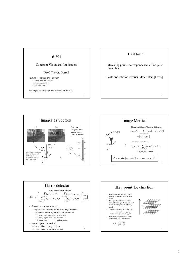
Images as Vectors
Left Right
L
w
R
w
m m L
w
L
w
row 1 row 2 row 3
m m m
“Unwrap” image to form vector, using raster scan order
Each window is a vector in an m2 dimensional vector space. Normalization makes them unit length.
4
Image Metrics
L
w ) (d wR
2 ) , ( ) , ( 2 SSD
) ( )] , ( ˆ ) , ( ˆ [ ) ( d w w v d u I v u I d C
R L y x W v u R L
m
− = − − =
∑
∈
(Normalized) Sum of Squared Differences Normalized Correlation
θ cos ) ( ) , ( ˆ ) , ( ˆ ) (
) , ( ) , ( NC
= ⋅ = − =
∑
∈
d w w v d u I v u I d C
R L y x W v u R L
m
) ( max arg ) ( min arg
2 *
d w w d w w d
R L d R L d
⋅ = − =
5
Harris detector
( )
∆ ∆ ∆ ∆ =
∑ ∑ ∑ ∑
∈ ∈ ∈ ∈
y x y x I y x I y x I y x I y x I y x I y x
W y x k k y W y x k k y k k x W y x k k y k k x W y x k k x
k k k k k k k k
) , ( 2 ) , ( ) , ( ) , ( 2
)) , ( ( ) , ( ) , ( ) , ( ) , ( )) , ( ( Auto-correlation matrix
- Auto-correlation matrix
– captures the structure of the local neighborhood – measure based on eigenvalues of this matrix
- 2 strong eigenvalues => interest point
- 1 strong eigenvalue => contour
- 0 eigenvalue => uniform region
- Interest point detection
– threshold on the eigenvalues – local maximum for localization
6
Key point localization
- Detect maxima and minima of
difference-of-Gaussian in scale space
- Fit a quadratic to surrounding
values for sub-pixel and sub-scale interpolation (Brown & Lowe, 2002)
- Taylor expansion around point:
- Offset of extremum (use finite
differences for derivatives):
B l u r