Latent Semantic Indexing Information Systems M Prof. Paolo Ciaccia - - PDF document

SLIDE 1

1

Latent Semantic Indexing

Information Systems M

• Prof. Paolo Ciaccia

http://www-db.deis.unibo.it/courses/SI-M/

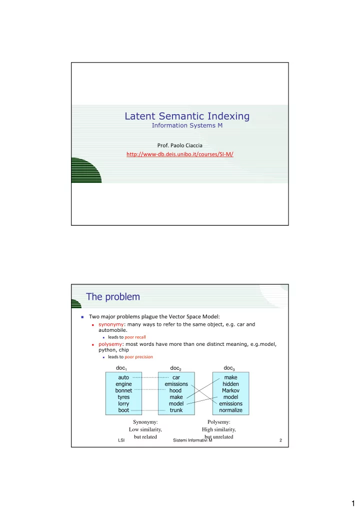
• Two major problems plague the Vector Space Model:
• synonymy: many ways to refer to the same object, e.g. car and

automobile.

leads to poor recall

• polysemy: most words have more than one distinct meaning, e.g.model,

python, chip

leads to poor precision

• Synonymy:

Low similarity, but related Polysemy: High similarity, but unrelated doc1 doc2 doc3

LSI Sistemi Informativi M 2

SLIDE 2

2

• Latent Semantic Indexing (LSI), also known as Latent Semantic Analysis (LSA)

when not applied to IR, was proposed at the end of 80’s as a way to solve such problem, http://lsi.argreenhouse.com/lsi/LSI.html

• The basic observation is that terms are an unreliable means to assess the

relevance of a document wrt to a query

• Because of synonymy and polysemy
• Thus, one would like to represent document using a more semantically

accurate way, i.e., in terms of “concepts”

• LSI achieves this by analyzing the whole term-document matrrix W,

and by projecting it in a lower-dimensional “latent” space spanned by relevant “concepts”

• More precisely, LSI uses a linear algebra technique, called Singular Value

Decomposition (SVD), before performing dimensionality reduction

LSI Sistemi Informativi M 3

• Given a square m×m matrix S, a non-null vector v is an eigenvector of S if

there exists a scalar λ, called the eigenvalue of v, such that:

• The linear transformation associated to S does not change the directions of

eigenvectors, which are just stretched/shrinked by an amount given by the corresponding eigenvalue

• There are at most m distinct eigenvalues, which are solutions of the

characteristic equation

• For each eigenvalue, there are infinite corresponding eigenvectors
• If is an eigenvector, so it is k, k ≠ 0
• Thus, we can consider normalized eigenvectors, ∥v

v v v∥=1

• Sv = λv

Det(S - λI) = 0

LSI Sistemi Informativi M 4

SLIDE 3

3

• If S is a real and symmetric matrix, then
• All its eigenvalues are real
• All the (normalized) eigenvectors of distinct eigenvalues are mutually
• rthogonal (thus, linearly independent)
• If S has m linearly independent eigenvectors, then it can be written as

where:

• Λ

Λ Λ Λ is a diagonal matrix, Λ Λ Λ Λ = diag(λ1, λ2,…, λm), with λ1 ≥ λ2 ≥ … ≥ λm

• The columns of are the corresponding eigenvectors of

U is a column-orthonormal matrix

LSI Sistemi Informativi M 5

      = 2 1 1 2 S

. 1 ) λ 2 ( | λI S |

2

= − − = −

1 λ ; 2 / 1 2 / 1 v 3 λ ; 2 / 1 2 / 1 v

2 2 1 1

=         − = =         =

S = UΛ Λ Λ ΛUT

∑

=

× × =

m 1 c c j, c c i, j i,

u λ u s

• LSI

Sistemi Informativi M 6

      −             − =       = 2 / 1 2 / 1 2 / 1 2 / 1 1 3 2 / 1 2 / 1 2 / 1 2 / 1 2 1 1 2 S

U UT

Λ Λ Λ Λ

1 2 / 1 2 / 3 2 / 1 1 2 / 1 2 / 1 3 2 / 1 u λ u u λ u u λ u s ; u λ u s

2,2 2 1,2 2,1 1 1,1 m 1 c c 2, c c 1, 1,2 m 1 c c j, c c i, j i,

= − = − × × + × × = × × + × × = × × = × × =

∑ ∑

= =

SLIDE 4

4

!

• Consider the M×N term-document weight matrix W
• If W has rank r ≤ min{M,N}, then W can be factorized as:

where:

• is an M×r column.orthonormal matrix (T =),
• Λ

Λ Λ Λ is an r×r diagonal matrix

• is an N×r column.orthonormal matrix (T =)
• Λ

Λ Λ Λ is also called the “concept matrix”

• T is the “term-concept similarity matrix”
• D is the “document-concept similarity matrix”

LSI Sistemi Informativi M 7

W = TΛ Λ Λ ΛDT

∑

=

× × =

r 1 c c j, c c i, j i,

d λ t w

• SVD represents both terms and documents using a set of latent concepts
• This just says that the weight of ti in docj is expressed as a

“linear combination of term-concept and doc-concept weights”

LSI Sistemi Informativi M 8

∑

=

× × =

r 1 c c j, c c i, j i,

d λ t w

SLIDE 5

5

"#$

• Consider the 12×9 weight matrix below, whose rank is r = 9, in which two

“groups” of documents are present

LSI Sistemi Informativi M 9 W C1 C2 C3 C4 C5 G1 G2 G3 G4 Human 1 1 Interface 1 1 Computer 1 1 User 1 1 1 System 1 1 2 Response 1 1 Time 1 1 EPS 1 1 Survey 1 1 Tree 1 1 1 Graph 1 1 1 Minors 1 1

"%$

• It is Λ

Λ Λ Λ = diag(3.34,2.54,2.35,1.64,1.50,1.31,0.85,0.56,0.35)

LSI Sistemi Informativi M 10

T 0.22

• 0.11

0.29

• 0.41
• 0.11
• 0.34

0.52

• 0.06
• 0.41

0.20

• 0.07

0.14

• 0.55

0.28 0.50

• 0.07
• 0.01
• 0.11

0.24 0.04

• 0.16
• 0.59
• 0.11
• 0.25
• 0.30

0.06 0.49 0.40 0.06

• 0.34

0.10 0.33 0.38 0.00 0.00 0.01 0.64

• 0.17

0.36 0.33

• 0.16
• 0.21
• 0.17

0.03 0.27 0.27 0.11

• 0.43

0.07 0.08

• 0.17

0.28

• 0.02
• 0.05

0.27 0.11

• 0.43

0.07 0.08

• 0.17

0.28

• 0.02
• 0.05

0.30

• 0.14

0.33 0.19 0.11 0.27 0.03

• 0.02
• 0.17

0.21 0.27

• 0.18
• 0.03
• 0.54

0.08

• 0.47
• 0.04
• 0.58

0.01 0.49 0.23 0.03 0.59

• 0.39
• 0.29

0.25

• 0.23

0.04 0.62 0.22 0.00

• 0.07

0.11 0.16

• 0.68

0.23 0.03 0.45 0.14

• 0.01
• 0.30

0.28 0.34 0.68 0.18 D 0.20

• 0.06

0.11

• 0.95

0.05 0.08 0.18

• 0.01 -0.06

0.61 0.17

• 0.50 -0.03 -0.21 -0.26 -0.43

0.05 0.24 0.46

• 0.13

0.21 0.04 0.38 0.72

• 0.24

0.01 0.02 0.54

• 0.23

0.57 0.27

• 0.21 -0.37

0.26

• 0.02 -0.08

0.28 0.11

• 0.51

0.15 0.33 0.03 0.67

• 0.06 -0.26

0.00 0.19 0.10 0.02 0.39

• 0.30 -0.34

0.45

• 0.62

0.01 0.44 0.19 0.02 0.35

• 0.21 -0.15 -0.76

0.02 0.02 0.62 0.25 0.01 0.15 0.00 0.25 0.45 0.52 0.08 0.53 0.08

• 0.03 -0.60

0.36 0.04

• 0.07 -0.45

SLIDE 6

6

!"#$

• Since both T and D are column-orthonormal matrices, it is
• T is the (real and symmetric) M×M term.term similarity matrix, and the

columns of are the eigenvectors of such matrix

• T is the N×N document.document similarity matrix, and the columns of

are the eigenvectors of such matrix

• Λ

Λ Λ Λ2 is a matrix with the eigenvalues of T (and T )

LSI Sistemi Informativi M 11

W WT = (TΛ Λ Λ ΛDT)(TΛ Λ Λ ΛDT)T = (TΛ Λ Λ ΛDT)(DΛ Λ Λ ΛTTT) = TΛ Λ Λ Λ2TT WT W = (DΛ Λ Λ ΛTTT)(TΛ Λ Λ ΛDT) = DΛ Λ Λ Λ2DT

!"%$

• Since it is

we can view this as a “projection” of documents (columns of W) in the r-dimensional “concept space” spanned by T columns (i.e., TT rows)

• In this space, documents are represented by the columns of Λ

Λ Λ ΛDT (i.e., rows of DΛ Λ Λ Λ)

• It follows that WT W = (DΛ

Λ Λ Λ)(Λ Λ Λ ΛDT) amounts to compute the similarity between documents as the inner product in this r-dimensional latent semantic space

• Similarly, in this space terms are represented by by the columns of Λ

Λ Λ ΛTT

LSI Sistemi Informativi M 12

TT W = Λ Λ Λ ΛDT

SLIDE 7

7

• Given a “target” dimensionality k (k ≪ r), one can obtain an optimal

approximation Wk of the W matrix by retaining only the k largest λc’s

• Among all the rank-k approximations, Wk is the one that minimizes the

Frobenius norm:

• Thus, now we have:
• Typical values of k are 100 - 300

LSI Sistemi Informativi M 13

norm Frobenius A A X W W

M 1 i N 1 j 2 j i, F F k :rank(X) X k

min ∑∑

= = =

= − =

Wk = TkΛ Λ Λ ΛkDk

T

"#$

• With k = 2 one obtains: Λ

Λ Λ Λ2 =diag(3.34,2.54)

LSI Sistemi Informativi M 14 T2 0.22

• 0.11

0.20

• 0.07

0.24 0.04 0.40 0.06 0.64

• 0.17

0.27 0.11 0.27 0.11 0.30

• 0.14

0.21 0.27 0.01 0.49 0.04 0.62 0.03 0.45 D2

T

0.20 0.61 0.46 0.54 0.28 0.00 0.01 0.02 0.08

• 0.06

0.17

• 0.13
• 0.23

0.11 0.19 0.44 0.62 0.53 W2 C1 C2 C3 C4 C5 G1 G2 G3 G4 Human 0.16 0.40 0.38 0.47 0.18

• 0.05
• 0.12
• 0.16
• 0.09

Interface 0.14 0.37 0.33 0.40 0.16

• 0.03
• 0.07
• 0.10
• 0.04

Computer 0.15 0.51 0.36 0.41 0.24 0.02 0.06 0.09 0.12 User 0.26 0.84 0.61 0.70 0.39 0.03 0.08 0.12 0.19 System 0.45 1.23 1.05 1.27 0.56

• 0.07
• 0.15
• 0.21
• 0.05

Response 0.16 0.58 0.38 0.42 0.28 0.06 0.13 0.19 0.22 Time 0.16 0.58 0.38 0.42 0.28 0.06 0.13 0.19 0.22 EPS 0.22 0.55 0.51 0.63 0.24

• 0.07
• 0.14
• 0.20
• 0.11

Survey 0.10 0.53 0.23 0.21 0.27 0.14 0.31 0.44 0.42 Tree

• 0.06

0.23

• 0.14 -0.27

0.14 0.24 0.55 0.77 0.66 Graph

• 0.06

0.34

• 0.15 -0.30

0.20 0.31 0.69 0.98 0.85 Minors

• 0.04

0.25

• 0.10 -0.21

0.15 0.22 0.50 0.71 0.62

SLIDE 8

8

&'

• Given a query q (M×1) column vector, in matrix notation the N inner

products of q and the documents are computed as that now becomes:

• Thus, the query vector is transformed into qTTk

(note that this is not anymore a sparse vector) Example: the query “Human computer interaction” corresponds to the vector qT = (1,0,1,0,0,0,0,0,0,0,0,0) This is transformed in the vector qTT2= (0.46, -0.07)

LSI Sistemi Informativi M 15

qTW = (qTT)(Λ Λ Λ ΛDT)

qTWk = (qTTk)(Λ Λ Λ ΛkDk

T)

"%$

• The matrix Λ

Λ Λ Λ2D2

T is (Λ

Λ Λ Λ2 =diag(3.34,2.54)):

• The figure shows how queries, documents and terms are distributed over

the 2-dimensional concept space

LSI Sistemi Informativi M 16

λ λ λ λ2D2

T

0.668 2.037 1.536 1.804 0.935 0.000 0.033 0.067 0.267

• 0.152 0.432 -0.330 -0.584 0.279

0.483 1.118 1.575 1.346

• 1
• 0.5

0.5 1 1.5 2 0.5 1 1.5 2 2.5 Terms Documents Query

SLIDE 9

9

"($

• After normalizing and computing the cosine similarity, it is obtained
• In general, it can be argued that if the document collection consists of k

“topics”, then LSI will produce a “good” rank-k approximation of W (good = low Frobenius error)

• In this case, the distance between documents related to a same topic will

decrease, whereas that between documents of different topics will increase

LSI Sistemi Informativi M 17

Cosine similarity C1 C2 C3 C4 C5 G1 G2 G3 G4 VSM 0.81 0.29 0.29 LSI 0.99 0.93 0.99 0.98 0.90

• 0.15 -0.12 -0.10

0.04

• There are many situations in which a feature-object matrix shows up:
• In IR, features = terms and objects = documents
• For instance, take:
• features = opinions
• bjects = users
• Then, LSI can bring together “similar users”
• Other examples: spam filtering for e-mails, cross-language retrieval,

modelling of human cognitive function, etc.

• It seems that also Google uses “some form” of LSI (“semantic search”),
• btained by prefixing terms with “~” (e.g., ~phone, ~humor)

LSI Sistemi Informativi M 18

SLIDE 10

10

• PROS
• Tends to improve the effectiveness of the retrieval process
• Decreases the dimensionality of vectors
• Good for machine learning, in which high dimensionality is a problem
• Dimensions have “semantics”

CONS

• Reduced vectors are not sparse anymore
• Expensive to compute, difficult to scale
• LSI does not solve the polysemy problem, since each term is represented as

a single point in the concept space (which is the weighted average of possible term meanings)

LSI Sistemi Informativi M 19

)

• http://web.eecs.utk.edu/research/lsi/
• http://lsi.research.telcordia.com/
• Online demo of LSI
• http://www.cs.brown.edu/~th/papers/Hofmann-SIGIR99.pdf
• Describes an evolution of LSI, called PLSI (Probabilistic LSI), aiming to

provide a more accurate description of documents in terms of laternt concepts

LSI Sistemi Informativi M 20