Lecture 4 Approach Langtons Investigation Investigate 1D CAs - - PDF document

Part 2: Cellular Automata 8/27/04 1

8/27/04 1

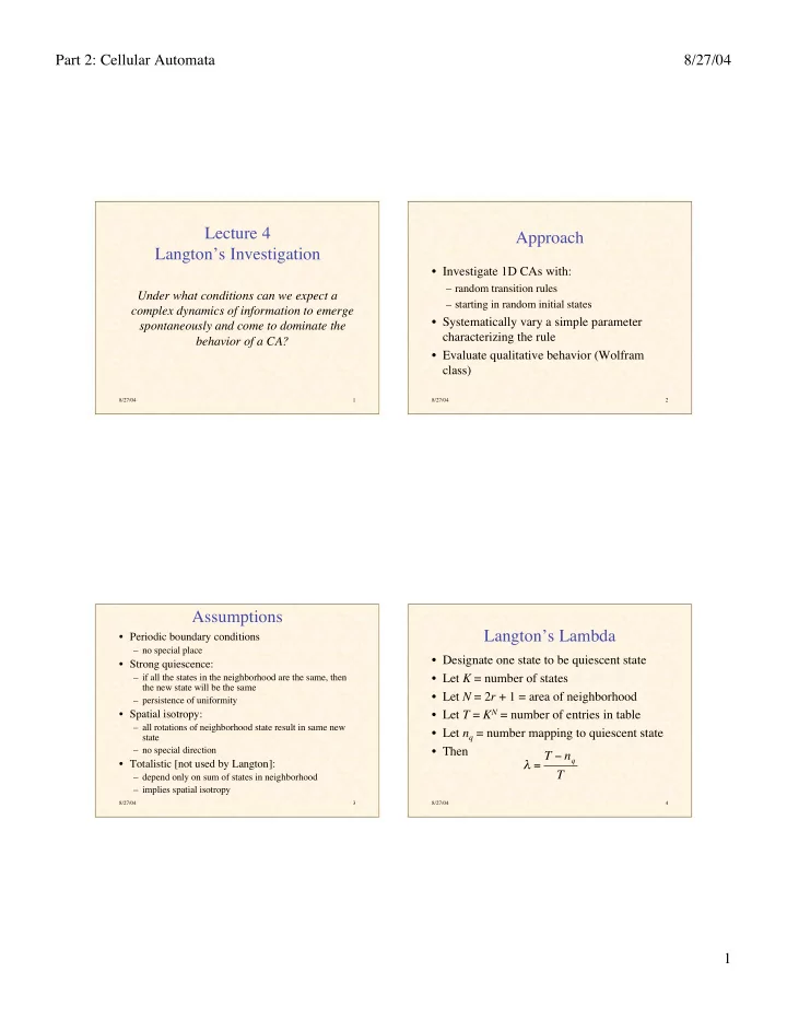
Lecture 4 Langton’s Investigation

Under what conditions can we expect a complex dynamics of information to emerge spontaneously and come to dominate the behavior of a CA?

8/27/04 2

Approach

• Investigate 1D CAs with:

– random transition rules – starting in random initial states

• Systematically vary a simple parameter

characterizing the rule

• Evaluate qualitative behavior (Wolfram

class)

8/27/04 3

Assumptions

• Periodic boundary conditions

– no special place

• Strong quiescence:

– if all the states in the neighborhood are the same, then the new state will be the same – persistence of uniformity

• Spatial isotropy:

– all rotations of neighborhood state result in same new state – no special direction

• Totalistic [not used by Langton]:

– depend only on sum of states in neighborhood – implies spatial isotropy

8/27/04 4

Langton’s Lambda

• Designate one state to be quiescent state
• Let K = number of states
• Let N = 2r + 1 = area of neighborhood
• Let T = KN = number of entries in table
• Let nq = number mapping to quiescent state
• Then

= T nq T

Part 2: Cellular Automata 8/27/04 2

8/27/04 5

Range of Lambda Parameter

• If all configurations map to quiescent state:

= 0

• If no configurations map to quiescent state:

= 1

• If every state is represented equally:

= 1 – 1/K

• A sort of measure of “excitability”

8/27/04 6

Example

• States: K = 5
• Radius: r = 1
• Initial state: random
• Transition function: random (given )

8/27/04 7

Class I ( = 0.2)

time

8/27/04 8

Class I ( = 0.2) Closeup

Part 2: Cellular Automata 8/27/04 3

8/27/04 9

Class II ( = 0.4)

8/27/04 10

Class II ( = 0.4) Closeup

8/27/04 11

Class II ( = 0.31)

8/27/04 12

Class II ( = 0.31) Closeup

Part 2: Cellular Automata 8/27/04 4

8/27/04 13

Class II ( = 0.37)

8/27/04 14

Class II ( = 0.37) Closeup

8/27/04 15

Class III ( = 0.5)

8/27/04 16

Class III ( = 0.5) Closeup

Part 2: Cellular Automata 8/27/04 5

8/27/04 17

Class IV ( = 0.35)

8/27/04 18

Class IV ( = 0.35) Closeup

8/27/04 19

Class IV ( = 0.34)

8/27/04 20

Part 2: Cellular Automata 8/27/04 6

8/27/04 21 8/27/04 22 8/27/04 23 8/27/04 24

Class IV Shows Some of the Characteristics of Computation

• Persistent, but not perpetual storage
• Terminating cyclic activity
• Global transfer of control/information

Part 2: Cellular Automata 8/27/04 7

8/27/04 25

• f Life
• For Life, 0.273
• which is near the critical region for CAs

with:

K = 2 N = 9

8/27/04 26

Transient Length (I, II)

8/27/04 27

Transient Length (III)

8/27/04 28

Shannon Information

(very briefly!)

• Information varies directly with surprise
• Information varies inversely with

probability

• Information is additive
• The information content of a message is

proportional to the negative log of its probability

I s

{ } = lgPr s { }

Part 2: Cellular Automata 8/27/04 8

8/27/04 29

Entropy

• Suppose have source S of symbols from

ensemble {s1, s2, …, sN}

• Average information per symbol:
• This is the entropy of the source:

Pr sk

{ }I sk { } =

k=1 N

• Pr sk

{ } lgPr sk { }

( )

k=1 N

• H S

{ } =

Pr sk

{ }lgPr sk { }

k=1 N

• 8/27/04

30

Maximum and Minimum Entropy

• Maximum entropy is achieved when all

signals are equally likely

No ability to guess; maximum surprise Hmax = lg N

• Minimum entropy occurs when one symbol

is certain and the others are impossible

No uncertainty; no surprise Hmin = 0

8/27/04 31

Entropy Examples

8/27/04 32

Entropy of Transition Rules

• Among other things, a way to measure the

uniformity of a distribution

• Distinction of quiescent state is arbitrary
• Let nk = number mapping into state k
• Then pk = nk / T

H = pi lg pi

i

• H = lgT 1

T nk lgnk

k=1 K

Part 2: Cellular Automata 8/27/04 9

8/27/04 33

Entropy Range

• Maximum entropy ( = 1 – 1/K):

uniform as possible all nk = T/K Hmax = lg K

• Minimum entropy ( = 0 or = 1):

non-uniform as possible

• ne ns = T

all other nr = 0 (r s) Hmin = 0

8/27/04 34

Further Investigations by Langton

• 2-D CAs
• K = 8
• N = 5
• 64 64 lattice
• periodic boundary conditions

8/27/04 35

• Avg. Transient Length vs.

(K=4, N=5)

8/27/04 36

• Avg. Cell Entropy vs.

(K=4, N=5)

H(A) = pk lg pk

k=1 K

Part 2: Cellular Automata 8/27/04 10

8/27/04 37

• Avg. Cell Entropy vs.

(K=4, N=5)

8/27/04 38

• Avg. Cell Entropy vs.

(K=4, N=5)

8/27/04 39

• Avg. Cell Entropy vs.

(K=4, N=5)

8/27/04 40

• Avg. Cell Entropy vs.

(K=4, N=5)

Part 2: Cellular Automata 8/27/04 11

8/27/04 41

• Avg. Cell Entropy vs.

(K=4, N=5)

8/27/04 42

Entropy of Independent Systems

• Suppose sources A and B are independent
• Let pj = Pr{aj} and qk = Pr{bk}
• Then Pr{aj, bk} = Pr{aj} Pr{bk} = pjqk

H(A,B) = Pr a j,bk

( )lgPr a j,bk ( )

j,k

• =

p jqk lg p jqk

( )

j,k

• =

p jqk lg p j + lgqk

( )

j,k

• =

p j lg p j

j

• +

qk lgqk

k

• = H(A) + H(B)

8/27/04 43

Mutual Information

• Mutual information measures the degree to

which two sources are not independent

• A measure of their correlation

I A,B

( ) = H A ( ) + H B ( ) H A,B ( )

• I(A,B) = 0 for completely independent

sources

• I(A,B) = H(A) = H(B) for completely

correlated sources

8/27/04 44

• Avg. Mutual Info vs.

(K=4, N=5)

I(A,B) = H(A) + H(B) – H(A,B)

Part 2: Cellular Automata 8/27/04 12

8/27/04 45

• Avg. Mutual Info vs.

(K=4, N=5)

8/27/04 46

Complexity vs.

8/27/04 47

Schematic of CA Rule Space vs.

• Fig. from Langton, “Life at Edge of Chaos”

8/27/04 48

Additional Bibliography

1. Langton, Christopher G. “Computation at the Edge of Chaos: Phase Transitions and Emergent Computation,” in Emergent Computation, ed. Stephanie Forrest. North-Holland, 1990. 2. Langton, Christopher G. “Life at the Edge of Chaos,” in Artificial Life II, ed. Langton et al. Addison-Wesley, 1992. 3. Emmeche, Claus. The Garden in the Machine: The Emerging Science of Artificial Life. Princeton, 1994.