[PDF] - Linear Programming Linear programming is the simplest form of PDF Document

SLIDE 1

Linear Programming

Linear programming is the simplest form of constrained optimization because the
bjective function is linear.
This implies that the minimum must lie on the boundary of the feasible region.
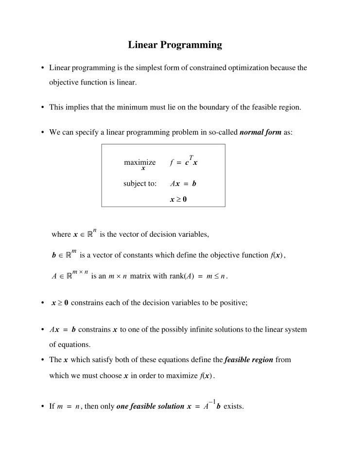
We can specify a linear programming problem in so-called normal form as:

maximize

x

f cTx = subject to: Ax b = x ≥ where x Rn ∈ is the vector of decision variables, b Rm ∈ is a vector of constants which define the objective function f x ( ), A Rm

n ×

∈ is an m n × matrix with rank A ( ) m n ≤ = .

x

≥

constrains each of the decision variables to be positive;

Ax

b =

constrains x to one of the possibly infinite solutions to the linear system

f equations.
The x which satisfy both of these equations define the feasible region from

which we must choose x in order to maximize f x ( ).

If m

n = , then only one feasible solution x A 1

– b

= exists.

SLIDE 2

If one also has inequality constraints given by

ai

Tx

bi ≤ then one can introduce “slack variables” such that: ai

Tx

xn

1 +

+ bi = xn

1 +

≥ This will add one more row to the matrix A, that is ai

T

ne more element b to the vector b, and
ne more decision variable xn

1 + to the vector of decision variables x.

In this way we can always convert a linear program with inequality constraints

into normal form by the addition of slack variables.

Also, if we were interested in the

minimization of f x ( ) instead, then we could maximize f x ( ) – That is, we would substitute c′ c – =

SLIDE 3

Example: Consider a factory in which there are three machines which we will denote as: M1 M2 M3 , , and which are used to make two products, P1 P2 , . For each unit of P1 made, machines M1 M2 , and M3 have to be run for 5, 3, and 4 minutes

respectively. For each unit of P2 the numbers are 1, 4, and 3 minutes. Every unit
f P1 produces a net profit of $30.00 while every unit of P2 produces $20.00 of
profit. We want to determine which production plan will give us the most profit?

Solution: Suppose we produce x1 units of P1 and x2 units of P2 per hour. Then the profit we want to maximize can be written as maximize

x

F 30x1 20x2 + = The constraints are that we cannot use any particular machine for more than 60 minutes per hour, that is: 5x1 x2 60 ≤ + (M1) 3x1 4x2 60 ≤ + (M2) 4x1 3x2 60 ≤ + (M3) x1 ≥ x2 ≥ We can now solve the problem graphically by first sketching the feasibility region in the x1 x2 , ( ) plane.

SLIDE 4

The feasibility region is shown shaded in the figure.
The level or contour lines for the objective functions are straight lines.
The maximum value will be attained at one of the corners of the boundary of the

feasible region.

The maximum of the objective function is attained at point B where its value is

F = 436.36. Found at the point where the two lines, labelled M1 and M3 intersect. 5x1 x2 + 60 = 4x1 3x2 + 60 = from which we get x∗ 10.9 5.5 , ( ) = .

3 6 9 12 15 3 6 9 15 12 18

x1 x2 3x1 4x2 + 60 =

M1

5x1 x2 + 60 = 4x1 3x2 + 60 =

M2 M3 A D C X B

F = 60 F = 120 F = 180 F = 240 F = 300 F = 360 F = 480 F = 436.36 F = 420

x3 = ( ) x4 = ( ) x5 = ( )

SLIDE 5

Graphical sketch of the problem.

This same problem can be written in normal form by introducing three slack

variables x3 x4 x5 , , (i.e. one for every inequality constraint).

Then we have:

maximize

x

F 30x1 20x2 + = subject to the new equality constrains: 5x1 x2 x3 + + 60 = 3x1 4x2 x4 + + 60 = 4x1 3x2 x5 + + 60 = ⎩ ⎪ ⎨ ⎪ ⎧ xi ≥ , i 1 … 5 , , =

The three equality constraints define a 2-D subspace of the 5-D space of the

problem (i.e. 5 - 3 = 2). Therefore, picking values for 2 of the variables, or coordinates, uniquely determines the remaining ones.

Each side of the feasible region in the original problem with the inequality

constraints has an equation of the form xi = . Specifically: x1 = (left side) x2 = (bottom) x3 = M1 ( ) x4 = M2 ( ) x5 = M3 ( )

SLIDE 6

Since a vertex of the boundary of the feasible region is the intersection of two

sides, therefore two of the variables are zero at a vertex point.

The vertices in the figure are defined as follows:

vertex 0: x1 x2 = = vertex A: x2 x3 = = vertex B: x3 x5 = = vertex C: x4 x5 = = vertex D: x1 x4 = = The vertex labeled X is defined by setting the two variables: x3 x4 = = but it is not a feasible point.

We can generalize these ideas by again considering a general linear programming

problem written in normal form maximize

x

f cTx = , x Rn ∈ , c Rn ∈ subject to: Ax b = , A Rm

n ×

∈ , b Rm ∈ x ≥

SLIDE 7

The m equations, Ax

b = , define an n m – ( ) dimensional subspace in the n dimensional space of the coordinates x.

This implies that n

m – ( ) coordinates may be chosen arbitrarily and these determine the remaining m coordinates.

A point satisfying the equations Ax

b = and x ≥ is called a feasible point or feasible vector. The feasible vectors define a “polyhedron” in the n m – ( ) dimensional space.

If n

m – ( ) of the n coordinates of a feasible vector are zero, then the vector is called a basic feasible vector. (These correspond to the vertices of the n m – ( )-dimensional polyhedron).

If more than n

m – ( ) coordinates are zero at a feasible vector, then the vector is called a degenerate feasible vector.

The optimal feasible vector (optimal solution) is the feasible vector at which the

function takes on the largest possible value in the feasible region. There may exist more than one optimal feasible vector; this is the case when the level lines of the function are parallel to one of the sides of the polyhedron. This implies that some optimal solution is not basic (i.e. not a vertex).

SLIDE 8

Theorem: Some optimal feasible vector is also a basic feasible vector - i.e. at least n m –

f

its coordinates are zero. (Geometrically, this means that an optimal feasible vector exists at one of the vertices of the polyhedron). The column vectors of the equation Ax b = corresponding to the non-zero coordinates are linearly independent.

Using this theorem, we can search for the optimal basic feasible vector by trying

all the n n m – ⎝ ⎠ ⎛ ⎞ n! n m – ( )!m!

=

combination of choosing n m – ( ) coordinates out of n to be zero. This is very inefficient!

SLIDE 9

Simplex Method

A more efficient method is to use what is called the simplex method.

It is an iterative search technique which, starting at one vertex, moves the search along the lines defining the polyhedron to another vertex only if the function increases at that new vertex. If no movement can be made, then the algorithm stops.

We explain the method by example. Consider the previous example in normal

form: maximize

x

F 30x1 20x2 + = , x R5 ∈ subject to: 5x1 x2 x3 + + 60 = 3x1 4x2 x4 + + 60 = 4x1 3x2 x5 + + 60 = ⎩ ⎪ ⎨ ⎪ ⎧ xi ≥ , i 1 … 5 , , = Step I: Look for a basic feasible vector at which to begin the search. We do this by choosing n m – ( ) right-hand variables which will be given a value

f zero and m left-hand variables whose value we will calculate using only the

right-hand variables. We also express the objective function using only the right-hand variables.

SLIDE 10

In our example, we have: x3 60 5x1 x2 – – = x4 60 3x1 – 4x2 – = x5 60 4x1 – 3x2 – = f 30x1 20x2 + = Here we have chosen x1 x2 = = and we note that at this point x3 ≥ , x4 ≥ , x5 ≥ . If these inequalities were not satisfied then we would have to choose a another vertex. Here, x1 x2 x3 ⇒ x4 x5 60 > = = = = = which means that we have a feasible point. Step II: Check the following maximum criterion. If none of the coefficients in the expression of f as a function of the present right-hand variables is positive, then the maximum criterion is satisfied. If any of the coefficients are positive, then increasing the right hand variable associated with that co-efficient increases f x ( ) which means that the maximum has not been found. If the coefficients are negative, this implies that the value of the function cannot be increased since the variables must remain positive, xi ≥ .

SLIDE 11

Step III: If maximum criterion is not fulfilled, determine the right hand variable which, when increased produces the greatest increase in f x ( ) while keeping all the left hand variables ≥ . For our example both right-hand variables x1 x2 , have positive coefficients. Looking at the first three equations and varying x1 and leaving x2 = we have: x3 ≥ if ∆x1 60 5

≤

12 = x4 ≥ if x1 ∆ 60 3

≤

20 = x5 ≥ if x1 ∆ 60 4

≤

15 = Thus, we can not increase x1 more than x1 ∆ 12 = . Varying x2 while keeping x1 = x3 ≥ if x2 ∆ 60 ≤ x4 ≥ if x2 ∆ 60 4

≤

15 = x5 ≥ if x2 ∆ 60 3

≤

20 = therefore we cannot increase x2 more than x2 ∆ 15 = .

SLIDE 12

This procedure can be shortened as follows: identify the right-hand variable in

the equality constraint equations which has a positive coefficient in f x ( ) and is allowed to increase the least. x3 60 5x1 – x2 – x1 ∆ ⇒ + 60 5

12

= = = f ∆ 30 ( ) 12 ( ) 360 = = x4 60 3x1 – 4x2 x2 ∆ ⇒ – 60 4

15

= = = f ∆ 20 ( ) 15 ( ) 300 = = x5 60 4x1 – 3x2 – = f 30x1 20x2 + =

Therefore, changing x1 by x1

∆ 12 = will give x3 = and produce the biggest increase in f .

This variable will now be the new right-hand variable which implies that we have

moved to a new vertex. Step IV: Exchange the right-hand variable, say xR, which gave the greatest value for f ∆ with the left-hand variable in the constraint equation where xR is identified.

SLIDE 13

Back to our example, we have x1 60 x3 – x2 – 5

=

which we substitute into the remaining equations: x1 12 1 5

– x2

1 5

– x3

+ + = x4 60 3 ( ) 12 ( ) – 3 5

x2

3 5

x3

4x2 – + + = x5 60 4 12 ( ) – 4 5

x2

x3 3x2 – + + = f 30 12 1 5

x2

– 1 5

–

⎝ ⎠ ⎛ ⎞ x3 20x2 + =

Now repeat steps II, III, and IV until the maximum criterion is satisfied.
Continuing with our example, we have

x1 12 1 5

x2

– 1 5

– x3

+ = x4 24 17 5

x2

– 3 5

x3

+ = x5 12 11 5

x2

– 4 5

x3

+ = x2 ∆ 60 11

=

f ∆ 14 ( ) 60 ( ) 11

840

11

=

= f 360 14x2 6x3 – + = Note, we only need to check x2 since the coefficient of x3 is negative. Now exchange x5 with x2:

SLIDE 14

x2 5 11

12

4 5

x3

x5 – + ⎝ ⎠ ⎛ ⎞ 60 4x3 5x5 – + 11

=

= x4 24 17 5

60

4x3 5x5 – + 11

–

3 5

x3

+ 60 7x3 – 17x5 + 11

=

= x1 120 3x3 – x5 + 11

=

f 4800 10x3 – 70x5 – 11

=
Since none of the coefficients of the new right-hand variables in f x

( ) are positive, this implies that the maximum criterion is fulfilled, which implies fmax 4 800 , 11

=

x∗ 120 11

60

11

0 60

11 , , , , ⎝ ⎠ ⎛ ⎞ = which is the vertex labeled B in our figure.

SLIDE 15

Some Special Cases Degenerate feasible vector

Recall that at a degenerate feasible vector, more than n

m –

f its coordinates are

zero.

Consider the following example:

maximize f 2x1 2x2 3x3 + + = subject to: x1 x3 + 1 ≤ x2 x3 + 1 ≤ xi ≥ i 1 2 3 , , =

The feasible region is pyramid shown and is defined by 5 vertices labelled 0, A,

B, C and D.

A D B C (0, 1, 0) (1, 1, 0) (1, 0, 0) (0, 0, 0) (0, 0, 1)

x3 x2 x2 x3 + 1 = x1 x3 + 1 = x5 = x4 = x1 Feasible region is inside a pyramid in three dimensional space.

SLIDE 16

We now introduce the slack variables x4 x5

, which in normal form gives us 5 variables and 2 equality constraints. Therefore we have n 5 = m 2 = ⎭ ⎬ ⎫n m – 3 = degrees of freedom.

The equality constraints become

x1 x3 x4 + + 1 = x2 x3 x5 + + 1 = Therefore, setting x4 = implies that x1 x3 + 1 = which is the plane defined by the vertices ABC. Setting x5 = means that x2 x3 + 1 = and this represents the plane defined by the vertices ABD.

The vertices are defined as follows:

at vertex 0: x1 x2 x3 = = = at vertex A: x1 x2 x4 x5 = = = = (degenerate) at vertex B: x3 x4 x5 = = = at vertex C: x2 x3 x4 = = = at vertex D: x1 x3 x5 = = =

SLIDE 17

Consider the initial basic feasible vector x1

x2 x3 = = = which implies the

rigin. If we choose these as the right-hand variables, we have

x4 1 = x1 x3 – – x1 ∆ 1 f ∆ , 2 = = x3 ∆ 1 f ∆ , 3 = = x5 1 x2 – x3 – = x2 ∆ 1 f ∆ , 2 = = x3 ∆ 1 f ∆ , 3 = = f 2x1 2x2 3x3 + + = Now x3 gives us the largest increase in f but it can be interchanged with either x4 or x5 since either interchange allows us to increase f by the same amount.

Say we choose to interchange x3 with x4. Then x1 x2 x4

, , ( ) will be the new right-hand variables which implies that we are at the vertex labelled A.

Algebraically, we have

x3 1 x1 – x4 – = x5 1 x2 – 1 x1 – x4 – ( ) – x1 x2 – x4 + = = x2 ∆ f ∆ , = = f 2x1 2x2 3 1 x1 – x4 – ( ) + + 3 x1 – 2x2 3x4 – + = = in which only x2 has a positive coefficient, but we are not allowed to increase x2 at all.

Therefore we exchange x2 and x5 and x1 x4 x5

, , ( ) become the new right-hand variables, but we are still at vertex A. This is because point A is a degenerate feasible vector: 0 0 1 0 0 , , , , ( ).

SLIDE 18

We now have:

x2 x1 = x4 x5 – + x3 1 x1 – x4 – = x1 ∆ 1 f ∆ , 1 = = f 3 x1 – 2 x1 x4 x5 – + ( ) 3x4 – + 3 x1 x4 – 2x5 – + = = and we exchange x1 and x3 making x3 x4 x5 , , ( ) the new right-hand variables which implies that we are now at vertex B.

This gives us the algebraic system:

x1 1 x3 – x4 – = x2 1 x3 – x4 – x4 x5 – + 1 x3 – x5 – = = f 3 1 x3 – x4 – x4 – 2x5 – + 4 x3 – 2x4 – 2x5 – = = and since all the coefficients are negative the maximum criterion is fulfilled.

We see that the optimal solution is given by

x∗ 1 1 0 0 0 , , , , ( ) = for which we have fmax 4 = .

Thus, we have seen that once we reach a degenerate feasible vector, it may take

more than one exchange of right-hand variables to left-hand variables in order to reach another basic feasible vector.

SLIDE 19

Difficulty in Finding Starting Points

A second difficulty may arise when the origin is not feasible. Now we may not

know how to find a basic feasible vector as a starting point. We demonstrate how to overcome this difficulty by example. Example: Consider the following problem: maximize f x1 x2 – = subject to: 2x1 x2 + 2 – ≤ – x1 2x2 – 2 ≤ x1 x2 + 5 ≤ xi ≥ i 1 2 , = The graph of this problem is shown below.

A B C D

x2 x1 2x1 – x2 + 2 – = x1 x2 + 5 = x5 = ( ) x1 2x2 – 2 = x4 = ( ) x3 = ( ) Feasible region is polygon enclosed by ABCD

SLIDE 20

Introducing the slack variables x3 x4 x5

, , we see that n 5 = , m 3 = and therefore we have n m – 2 = degrees of freedom (i.e. 2 right-hand variables). In normal form the problem is written as: f x1 x2 – = 2x1 – x2 x3 + + 2 – = x1 2x2 – x4 + 2 = x1 x2 x5 + + 5 = xi ≥ i 1 2 3 4 5 , , , , = ( ) Now we notice that the origin x1 = , x2 = is not feasible!

A general technique to find a starting point is the introduction of a new artificial
variable. Notice that if we tried to use the origin as the first basic feasible vector

then we would get the system x3 2 – 2x1 x2 – + = x4 2 x1 – 2x2 + = x5 5 x1 – x2 – = and since the right-hand variables are set to zero, that is x1 x2 = = , we would have x3 2 – < = which violates the xi ≥ constraint.

SLIDE 21

We now introduce the artificial variable x6

≥ in the offending equation. The number of equations remains the same but the number of variables has increased by 1, therefore we can set n 1 + ( ) m – n m – ( ) 1 + = variables equal to zero. We add the artificial variable to the equation x3 2 – 2x1 x2 – x6 + + = and move the new variable to the left x6 2 2x1 – x2 x3 + + =

Now choosing x1 x2 x3

, , ( ) as the right-hand variables, we will have x6 ≥ which is feasible. In the final solution we require that x6 = and this will imply that 2 – 2x1 x2 – + x3 = . To ensure this we modify the objective function as: f ˆ x1 x2 – Mx6 – = where M is a very large positive number.

Therefore, in order to maximize this, we require x6

→ , and in terms of the right-hand variables: x6 2 2x1 – x2 x3 + + = x1 ∆ 1 f ∆ , 1 2M + = = x4 2 x1 – 2x2 + = x5 5 x1 – x2 – = f ˆ x1 x2 – M 2 2x1 – x2 x3 + + ( ) – 1 2M + ( )x1 1 M + ( )x2 Mx3 – 2M – – = =

SLIDE 22

Now we see that only the variable x1 has a positive coefficient. We exchange x1

and x6 and get x1 2 x2 x3 x6 – + + 2

=

x4 2 1 1 2

x2

1 2

x3

1 2

x6

– + + 2x2 + – 1 3 2

x2

1 2

x3

– 1 2

x6

+ + = = x5 5 1 1 2

x2

1 2

x3

1 2

x6

– + + – x2 – 4 3 2

x2

– 1 2

x3

– 1 2

x6

+ = = f ˆ 1 2M + ( ) 1 1 2

x2

1 2

x3

1 2

x6

– + + 1 M + ( )x2 – Mx3 – 2M – = 1 1 2

x2

– 1 2

x3

1 2

x6

– Mx6 – + =

Now since x6 has become the right hand variable, it can be set to zero and
removed. The new right-hand variables are x2 and x3 which implies point A. We

have x1 1 x2 2

x3

2

+

+ = x4 1 3 2

x2

1 2

x3

– + = x3 ∆ 2 f ∆ , 1 = = x5 4 3 2

x2

– 1 2

x3

– = f 1 1 2

x2

– 1 2

x3

+ =

SLIDE 23

We exchange x3 and x4: right hand variables x2 x4

, which implies Point B. x3 2 3x2 2x4 – + = x1 1 1 2

x2

1 2

2

3x2 2x4 – + [ ] + + 2 2x2 x4 – + = = x5 4 3 2

x2

– 1 2

2

3x2 2x4 – + [ ] – 3 3x2 – x4 + = = x2 ∆ 1 f ∆ , 1 = = f 1 1 2

x2

– 1 2

2

3x2 2x4 – + [ ] + 2 x2 x4 – + = =

We exchange x2 and x5 and the right-hand variables become x4 x5

, which implies point C. x2 1 1 3

x4

– 1 3

x5

– = x3 2 3 1 1 3

x4

– 1 3

x5

– 2x4 – + 5 3x4 – x5 – = = x1 2 2 1 1 3

x4

– 1 3

x5

– x4 – + 4 5 3

x4

– 2 3

x5

– = = f 2 1 1 3

x4

– 1 3

x5

– x4 – + 3 4 3

x4

– 1 3

x5

– = =

Since all the coefficients are negative, the maximum criterion is satisfied and we

have fmax 3 = at 4 1 5 0 0 , , , , ( ) which is point C.

SLIDE 24

Multiple Optimal Solutions:

If the level lines of the objective function are parallel to one of the sides of the

feasible region, then a multiple optimal solution will occur along that side. Of course, there is still only one value for fmax and fmin.

This condition will manifest itself algebraically by the absence of one or more of

the right-hand variables in the final form of the objective function.

SLIDE 25

Example: Optimal Utilization of a Communications Network

It is quite remarkable to find such a large number of applications which can be

formulated as a linear program.

Consider a communications network in which we have:

1) N stations in which messages are sent, relayed, and received; 2) a set of links connecting the stations over which the messages travel; and 3) a set of messages.

The following notation and terminology is now used:

T is the interval of time over which messages are sent, received and relayed. aij are the demand coefficients which represent the number of messages

riginating at station i per time T and destined for another station j.

cij is the capacity of the direct link from station i to j during period T. si is the switching capacity at station i during the time interval T. (i.e. number of messages entering and leaving the ith node during T cannot exceed si. xijk is the number of messages sent from station i (not necessarily originating at i) over one link to another station j during T and destined for k i ≠ . xiik = ik ∀ combinations xiji = ij ∀ combinations P1 is the ratio of the number of delivered messages to the number of originating messages during T.

The optimal routing or utilization problem tries to optimize P1

SLIDE 26

Therefore we can write the objective function as maximize

x

P1 xijj

i j ,

∑

aij

i j ,

∑

=

where xijj is the number of messages which have been delivered.

We have an inequality constraint related to the demand for messages

ximj

m

∑

xmij

m

∑

– aij ≤ i j , ∀ i j ≠ where ximj are the messages sent from i to m and destined for j and xmij are the messages sent from m to i and destined for j. The first term on the left of the inequality represents the total number of messages sent out from i and destined for j. The second term represents the total number of messages coming into i destined for j from all other nodes.

SLIDE 27

The total number of messages sent out from i and destined for j must be less than

the total number of messages originating at i plus the messages using i as an intermediate node with j as the destination node. aij ximj

m

∑

xmij

m

∑

i

destination node

j

rest of network

Demand limitation constraint.

The next set of inequalities are related to link capacity:

xijk

k

∑

cij ≤ i j , ∀ i j ≠

switching centre capacity for messages leaving node i:

xijk

j k ,

∑

si ≤ i ∀

and switching centre capacity for messages entering node i:

xkij

j k ,

∑

si ≤ i ∀ .

SLIDE 28

2 1 3

S1 (capacity of station 1)

demand coefficients

a12 a13 ⎩ ⎭ ⎨ ⎬ ⎧ ⎫ C31

(link capacity)

S3 S2 C23 C13 C13 C21

(capacity of station 3)

a21 a23 ⎩ ⎭ ⎨ ⎬ ⎧ ⎫ C32 a31 a32 ⎩ ⎭ ⎨ ⎬ ⎧ ⎫ Example network with three nodes.

The linear program associated with this network can be written as

maximize

x

P1 x122 x133 x211 x233 x311 x322 + + + + + a12 a13 a21 a23 a31 a32 + + + + +

=

subject to the demand constraints: x122 x132 x312 – + a12 ≤ x123 x133 x213 – + a13 ≤ x231 x211 x321 – + a21 ≤ x233 x213 x123 – + a23 ≤ x311 x321 x231 – + a31 ≤ x312 x322 x132 – + a32 ≤

SLIDE 29

the link capacity constraints:

x122 x123 + C12 ≤ x132 x133 + C13 ≤ x211 x213 + C21 ≤ x231 x233 + C23 ≤ x311 x312 + C31 ≤ x321 x322 + C32 ≤

switch capacity constraints for messages leaving each node

x122 x123 x132 x133 + + + S1 ≤ x211 x213 x231 x233 + + + S2 ≤ x311 x312 x321 x322 + + + S3 ≤

and switch capacity constraints for messages entering each node

x211 x213 x311 x312 + + + S1 ≤ x122 x123 x321 x322 + + + S2 ≤

The message demands, aij, may change depending on the time period (business

hours, night time, etc.) therefore, the decision on how to choose xijk so as to maximize P1 may have to be determined many times a day from estimates of the demands.

SLIDE 30

2 1 3

S1 5 = a12 2 = a13 1 = ⎩ ⎭ ⎨ ⎬ ⎧ ⎫

C31 2 =

S3 6 = S2 4 =

C23 2 =

C13 3 =

C12 3 =

C21 1 = a21 1 = a23 2 = ⎩ ⎭ ⎨ ⎬ ⎧ ⎫ C32 2 = a31 2 = a32 2 = ⎩ ⎭ ⎨ ⎬ ⎧ ⎫ Specific network with three nodes.

The variables are:

x x122 x132 x123 x133 x211 x231 x233 x213 x311 x321 x322 x312 = and the linear program is written as maximize

x

P1 x122 x133 x211 x233 x311 x322 + + + + + a12 a13 a21 a23 a31 a32 + + + + +

=

that is maximize

x

P1 1 10

x122

x133 x211 x233 x311 x322 + + + + + ( ) =

SLIDE 31

The next equations are the demand limitation constraints:

i 1 =

, j

2 =

, x122

x132 + x312 – 2 ≤ i 1 =

, j

3 =

, x123

x133 + x213 – 1 ≤ i 2 =

, j

1 =

, x211

x231 + x321 – 1 ≤ i 2 =

, j

3 =

, x213

x233 + x123 – 2 ≤ i 3 =

, j

1 =

, x311

x321 + x231 – 2 ≤ i 3 =

, j

2 =

, x312

x322 + x132 – 2 ≤ the link capacity constraints x122 x123 + C12 ≤ 3 = x132 x133 + C13 ≤ 3 = x211 x213 + C21 ≤ 1 = x231 x233 + C23 ≤ 2 = x311 x312 + C31 ≤ 2 = x321 x322 + C32 ≤ 2 = the switch capacity constraints for messages leaving each node x122 x123 x132 x133 + + + S1 ≤ 5 = x211 x213 x231 x233 + + + S2 ≤ 4 = x311 x312 x321 x322 + + + S3 ≤ 6 = and the switch capacity constraints for messages entering each node x211 x213 x311 x312 + + + S1 ≤ 5 = x122 x123 x321 x322 + + + S2 ≤ 4 = x131 x132 x231 x233 + + + S3 ≤ 6 =

SLIDE 32

Another Look at Basic Solutions

Recall that a linear program can be written in normal or standard form.

minimize

x

f cTx =

,

x Rn ∈

, c

Rn ∈ subject to: Ax b = , A Rm

n ×

∈ , b Rm ∈ x ≥ with m n < , rank A m = , and b ≥ . Now consider the equality constraints Ax b = .

Let B be an mxm matrix whose columns are linearly independent, and re-write:

A B D , [ ] = where D is a m m n – ( ) ×

matrix. Since the matrix B is non-singular we can

write BxB b =

, xB

Rm ∈ and xB B 1

– b

=

.

If we let

x xB = then x is a solution of Ax b = . We now make the following definitions:

SLIDE 33

Definitions

x

xB 0

T

= Rn ∈ is a basic solution of Ax b = with respect to the basis B. The components of xB are called basic variables, (or left hand variables). The columns of B are called basic columns.

if some basic variables of a basic solution are zero then the solution is called a

degenerate basic solution.

if x satisfies Ax

b = and x ≥ then x is called a feasible solution.

if a feasible solution is also basic it is called a basic feasible solution.
if a basic feasible solution is also degenerate then we call it a degenerate basic

feasible solution. Consider the problem defined by A 2 3 1 – 1 – 4 1 1 2 – =

, b

1 – 9 = and form the augmented matrix A b , [ ]: A b , [ ] 2 3 1 – 1 – 1 – 4 1 1 2 – 9 = we now perform elementary row operations to get 1 0 2 5 ⁄ 1 – 2 ⁄ 14 5 ⁄ 0 1 3 – 5 ⁄ 11 – 5 ⁄

.

SLIDE 34

This implies that the general solution can be written with two parameters,

s t R ∈ , , as x1 14 5

=

2 5

s

– 1 2

t

+ x2 11 5

–

3 5

s

+ = x3 s = x4 t = x 14 5 ⁄ 11 – 5 ⁄ ⎝ ⎠ ⎜ ⎟ ⎜ ⎟ ⎜ ⎟ ⎜ ⎟ ⎛ ⎞ s 2 – 5 ⁄ 3 5 ⁄ 1 ⎝ ⎠ ⎜ ⎟ ⎜ ⎟ ⎜ ⎟ ⎜ ⎟ ⎛ ⎞ + = t 1 2 ⁄ 1 ⎝ ⎠ ⎜ ⎟ ⎜ ⎟ ⎜ ⎟ ⎜ ⎟ ⎛ ⎞ +

Note that x

v h + = where v 14 5 ⁄ 11 – 5 ⁄ ⎝ ⎠ ⎜ ⎟ ⎜ ⎟ ⎜ ⎟ ⎜ ⎟ ⎛ ⎞ = h s 2 – 5 ⁄ 3 5 ⁄ 1 ⎝ ⎠ ⎜ ⎟ ⎜ ⎟ ⎜ ⎟ ⎜ ⎟ ⎛ ⎞ = t 1 2 ⁄ 1 ⎝ ⎠ ⎜ ⎟ ⎜ ⎟ ⎜ ⎟ ⎜ ⎟ ⎛ ⎞ + with Av b = , Ah = . We say that h is in the null space of A. We now can set the parameters so as to make any two elements of x equal to 0. There are six ways we can do this.

SLIDE 35

1) If we choose s t = = then we have x3 x4 = = which implies the basis is B a1 a2 , [ ] = which is the same as solving: 2 3 4 1 x1 x2 1 – 9 = x1 x2 ⇒ 14 5 ⁄ 11 – 5 ⁄ = which is a basic solution, but since x2 < this is not a basic feasible solution. 2) If we choose s and t such as to set x2 x4 = = then this implies that the basis is B a1 a3 , [ ] = which is the same as solving: 2 1 – 4 1 x1 x3 1 – 9 = x1 x3 ⇒ 4 3 ⁄ 11 3 ⁄ = which is a basic feasible solution. 3) If we choose s and t such as to set x2 x3 = = then this implies that B a1 a4 2 1 – 4 2 – = = which is singular and therefore B is not a basis. 4) If we choose s and t such as to set x1 x4 B ⇒ a2 a3 , = = = then we get x 2 7 ⎝ ⎠ ⎜ ⎟ ⎜ ⎟ ⎜ ⎟ ⎜ ⎟ ⎛ ⎞ = which is basic feasible.

SLIDE 36

5) If we choose s and t such as to set x1 x3 B ⇒ a2 a4 , [ ] = = = , then we get x 11 – 5 ⁄ 28 – 5 ⁄ ⎝ ⎠ ⎜ ⎟ ⎜ ⎟ ⎜ ⎟ ⎜ ⎟ ⎛ ⎞ = which is basic but not feasible. 6) If we choose s and t such as to set x1 x2 B ⇒ a3 a4 , [ ] = = = , then we get x 11 3 ⁄ 8 – 3 ⁄ ⎝ ⎠ ⎜ ⎟ ⎜ ⎟ ⎜ ⎟ ⎜ ⎟ ⎛ ⎞ = which is basic but not feasible.

Notice that the number of ways we can choose 2 elements of x to be zero given

that it has 4 elements is 4 2 ⎝ ⎠ ⎛ ⎞ 4! 2!2!

6

= = choices; or more generally n n m – ⎝ ⎠ ⎛ ⎞ n m ⎝ ⎠ ⎛ ⎞ = . Definitions

any x which minimizes the objective function cTx and satisfies the constraints

Ax b = , A Rm

n ×

∈ and x ≥ is said to be an optimal feasible solution.

an optimal feasible solution which is basic is said to be an optimal basic feasible

solution.

SLIDE 37

Theorem: fundamental theorem of linear program.

given a linear program in standard form:

if there exists a feasible solution, then there exists is a basic feasible solution.
if there exists an optimal feasible solution, then there exists an optimal basic