[PDF] - Logistic Regression Two Worlds: Probabilistic & Algorithmic We PDF Document

SLIDE 1

1

Logistic Regression

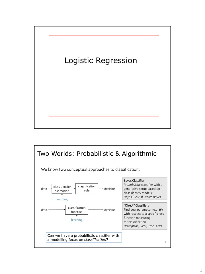
Two Worlds: Probabilistic & Algorithmic

Can we have a probabilistic classifier with a modelling focus on classification? Bayes es Classi ssifier er Probabilistic classifier with a generative setup based on class density models Bayes (Gauss), Naïve Bayes “Direct” Classifiers Find best parameter (e.g. 𝑥) with respect to a specific loss function measuring misclassification Perceptron, SVM, Tree, ANN

We know two conceptual approaches to classification:

data class density estimation classification rule decision learning data classification function decision learning

4

SLIDE 2

2

Advantages of Both Worlds

Posterior distribution has advantages over classification label:
Asymmetric risks: need classification probability
Classification certainty: Indicator if decision in unsure
Algorithmic approach with direct learning has advantages:
Focus of modelling power on correct classification where it counts
Easier decision line interpretation
Combination?

5

Discriminative Probabilistic Classifier

𝑄 𝑦 𝐷1 𝑄 𝑦 𝐷2

𝑕 Ԧ 𝑦 = 𝒙𝑈𝒚 + 𝑥0 𝑄 𝐷2 𝑦 ∝ 𝑄 𝑦 𝐷2 𝑄 𝐷2 Bayes Classifier Linear Classifier

6

Discriminative Probabilistic Classifier

Bishop PRML Bishop PRML

SLIDE 3

3

Towards a “Direct” Probabilistic Classifier

Idea 1: Directly learn a posterior distribution

For classification with the Bayes classifier, the posterior distribution is

relevant. We can directly estimate a model of this distribution (we called this

as a discriminative classifier in Naïve Bayes). We know from Naïve Bayes that we can probably expect a good performance from the posterior model.

Idea 2: Extend linear classification with probabilistic interpretation

The linear classifier outputs a distance to the decision plane. We can use this value and interpret it probabilistically: “The further away, the more certain”

7

Logistic Regression

The Logistic Regression will implement both ideas: It is a model of a posterior class distribution for classification and can be interpreted as a probabilistic linear classifier. But it is a fully probabilistic model, not only a “post-processing” of a linear classifier. It extends the hyperplane decision idea to Bayes world

Direct model of the posterior for classification
Probabilistic model (classification according to a probability distribution)
Discriminative model (models posterior rather than likelihood and prior)
Linear model for classification
Simple and accessible (we can understand that)
We can study the relation to other linear classifiers, i.e. SVM

8

SLIDE 4

4

History of Logistic Regression

Logistic Regression is a very “old” method of statistical analysis

and in widespread use, especially in the traditional statistical community (not machine learning).

1957/58, Walker, Duncan, Cox

A method more often used to study and identify explaining factors

rather than to do individual prediction.

Statistical analysis vs. prediction focus of modern machine learning Many medical studies of risk factors etc. are based on logistic regression

9

10

Statistical Data Models

Simplest form besides constant (one prototype) is a linear model.

 

1

,

d T w i i i

Lin x w x w w x w w x w



     



► Linear Methods: Classification: Logistic Regression (no typo!) Regression: Linear Regression

1 , w x w x w              

 

, ,

w

Lin x w x w w x    

We do not know P(x,y) but we can assume a certain form.

--> This is called a data model.

SLIDE 5

5

Repetition: Linear Classifier

Linear classification rule:

11

𝑕 𝒚 = 𝒙𝑈𝒚 + 𝑥0 𝑕 𝒚 ≥ 0 ⇒ 𝑕 𝒚 < 0 ⇒

Decision boundary is a a hyperplane

Repetition: Posterior Distribution

Classification with Posterior distribution: Bayes

Based on class densities and a prior

12

𝑄 𝐷2 𝒚 = 𝑞 𝒚 𝐷2 𝑄 𝐷2 𝑞 𝒚 𝐷1 𝑄 𝐷1 + 𝑞 𝒚 𝐷2 𝑄 𝐷2 𝑄 𝐷1 𝒚 = 𝑞 𝒚 𝐷1 𝑄 𝐷1 𝑞 𝒚 𝐷1 𝑄 𝐷1 + 𝑞 𝒚 𝐷2 𝑄 𝐷2

Bishop PRML

SLIDE 6

6

Combination: Discriminative Classifier

13

Probabilistic interpretation of classification

utput: ~distance to separation plane

Decision boundary

Bishop PRML

Notation Changes

We work with two classes

Data with (numerical) feature vectors Ԧ 𝑦 and labels 𝒛 ∈ {𝟏, 𝟐} We do not use the notation of Bayes with 𝜕 anymore. We will need the explicit label value of 𝒛 in our models later.

Classification goal: infer the best class label {𝟏 𝒑𝒔 𝟐} for a given feature point

𝑧∗ = arg max

𝑧∈{0,1} 𝑄(𝑧|𝒚)

All our modeling focuses only on the posterior of having class 1:

𝑄 𝑧 = 1 𝒚

Obtaining the other is trivial: 𝑄 𝑧 = 0 𝒚

= 1 − 𝑄(𝑧 = 1 |𝒚 )

14

SLIDE 7

7

Parametric Posterior Model

We need a model for the posterior distribution, depending on the feature vector (of course) and neatly parameterized. The linear classifier is a good starting point. We know its parametrization very well: We thus model the posterior as a function of the linear classifier:

Posterior from classification result: “scaled distance“ to decision plane

𝑄 𝑧 = 1 𝒚, 𝜾 = 𝑔 𝒚; 𝜾 𝑕 𝒚; 𝒙, 𝑥0 = 𝒙𝑈𝒚 + 𝑥0 𝑄 𝑧 = 1 𝒚, 𝒙, 𝑥0 = 𝑔(𝒙𝑈𝒚 + 𝑥0)

15

Logistic Function

To use the unbounded distance to the decision plane in a probabilistic setup, we need to map it into the interval [0, 1]

This is very similar as we did in neural nets: activation function

The logistic function 𝜏 𝑦 squashes a value 𝑦 ∈ ℝ to 0, 1 𝜏 𝑦 = 1 1 + e−𝑦

The logistic function is a smooth, soft threshold 𝜏 𝑦 → 1 𝑦 → ∞ 𝜏 𝑦 → 0 𝑦 → −∞ 𝜏 0 = 1

2

16

SLIDE 8

8

17

The Logistic Function

18

The Logistic “Regression”

SLIDE 9

9

The Logistic Regression Posterior

We model the posterior distribution for classification in a two- classes-setting by applying the logistic function to the linear classifier: 𝑄 𝑧 = 1 𝑦 = 𝜏 𝑕 𝑦 𝑄 𝑧 = 1 𝒚, 𝒙, 𝑥0 = 𝑔(𝒙𝑈𝒚 + 𝑥0) = 1 1 + 𝑓−(𝒙𝑈𝒚+𝑥0)

This a location-dependent model of the posterior distribution, parametrized by a linear hyperplane classifier.

19

Logistic Regression is a Linear Classifier

The logistic regression posterior leads to a linear classifier:

20

𝑄 𝑧 = 1 𝒚, 𝒙, 𝑥0 = 1 1 + exp −(𝒙𝑈𝒚 + 𝑥0) 𝑄 𝑧 = 0 𝒚, 𝒙, 𝑥0 = 1 − 𝑄 𝑧 = 1 𝒚, 𝒙, 𝑥0 𝑄 𝑧 = 1 𝒚, 𝒙, 𝑥0 > 1 2 ⇒ Classification boundary is at:

⇒ 1 1 + exp −(𝒙𝑈𝒚 + 𝑥0) = 1 2

𝒙𝑈𝒚 + 𝑥0 = 0

𝑧 = 1 classification; 𝑧 = 0 otherwise

𝑄 𝑧 = 1 𝒚, 𝒙, 𝑥0 = 1 2

Classification boundary is a hyperplane

⇒

SLIDE 10

10

Interpretation: Logit

Is the choice of the logistic function justified?

Yes, the logit is a linear function of our data:

Logit: log of the odds ratio: ln

𝑞 1−𝑞

But other choices are valid, too

They lead to other models than logistic regression, e.g. probit regression → Generalized Linear Models (GLM)

21

ln 𝑄(𝑧 = 1|𝒚) 𝑄(𝑧 = 0|𝒚) = 𝒙𝑈𝒚 + 𝑥0

The linear function (~distance from decision plane) directly expresses our classification certainty, measured by the “odds ratio”: double distance ↔ squared odds e.g. 3: 2 → 9: 4

𝐹[𝑧] = 𝑔−1 𝒙𝑈𝒚 + 𝑥0

22

The Logistic Regression

So far we have made no assumption on the data!
We can get r(x) from a generative model or model it

directly as function of the data (discriminative)

Logistic Regression:

Model: The logit r(x) = log

𝑄(𝑧=1|𝒚) 𝑄(𝑧=0|𝒚) = log 𝑞 1−𝑞

is a linear function of the data < = >

 

1

log , 1

d i i i

p r x w x w w x p



    



   

1 , P y x w x   

     

1 1 , 1 exp , P y x w x w x      

SLIDE 11

11

Training a Posterior Distribution Model

The posterior model for classification requires training. Logistic regression is not just a post-processing of a linear classifier. Learning

f good parameter values needs be done with respect to the

probabilistic meaning of the posterior distribution.

In the probabilistic setting, learning is usually estimation

We now have a slightly different situation than with Bayes: We do not need class densities but a good posterior distribution.

We will use Maximum Likelihood and Maximum-A-Posteriori

estimates of our parameters 𝒙, 𝑥0

Later: This also corresponds to a cost function of obtaining 𝒙, 𝑥0

23

Maximum Likelihood Learning

The Maximum Likelihood principle can be adapted to fit the posterior distribution (discriminative case):

We choose the parameters 𝒙, 𝑥0 which maximize the posterior

distribution of the training set 𝒀 with labels 𝒁: 𝑄 𝑧 𝒚; 𝒙, 𝑥0 = 𝑄 𝑧 = 1 𝒚; 𝒙, 𝑥0 𝑧 𝑄 𝑧 = 0 𝒚; 𝒙, 𝑥0 1−𝑧 𝒙, 𝑥0 = arg max

𝒙,𝑥0 𝑄

Y 𝑌; 𝒙, 𝑥0 = arg max

𝒙,𝑥0

ς𝒚∈𝑌 𝑄 𝑧 𝒚; 𝒙, 𝑥0

(iid)

24

SLIDE 12

12

25

Logistic Regression: Maximum Likelihood Estimate of w

(1)

To simplify the notation we use w, x instead of 𝒙, 𝑥0

The discriminative (log) likelihood function for our data

   

1 N i

i i

P Y X P y x



 

     

1 1

1 (1 )

y y y y

P y x P y x P y x p p

 

     

1

(1 )

i i

N i

y y i i

p p





 



 

log P Y X 

 

1

log log 1 1

N i i i i i

p y p p



         



     

1

log 1 log 1

N i i i i i

y p y p



  



   

1

T

P y x w x   

   

1

T

P y x w x    

With and

“cross-entropy” cost function

26

log-likelihood function continued

 

log , log L Y X P Y X  

 

1

log log 1 1

N i i i i i

p y p p



        



 

1

log , log 1

N T i i i T i

w x

L Y X y w x e



  



Maximize the log-likelihood function with respect to w

 

log , L Y X w   

!

Maximum Likelihood Estimate of w (2)

 

1 1

T

T i w x

p w x e 



   Remember and linear Logit

l𝑝𝑕 𝑞𝑗 1 − 𝑞𝑗 = 𝑥𝑈𝑦

SLIDE 13

13

 

1

log , log 1

N T i i i T i

w x

L Y X y w x e w w



       

1

N T T i i i i T i T i

w x w x

e y x x e



  



Maximum Likelihood Estimate of w (3)

27

Derivative of a Dot Product

𝜖 𝜖𝒙 = 𝛼

𝐱 =

𝜖 𝜖𝑥1 , 𝜖 𝜖𝑥2 , … , 𝜖 𝜖𝑥𝑒 𝜖 𝜖𝒙 𝒙𝑈𝒚 = 𝜖 𝜖𝑥1 𝒙𝑈𝒚, 𝜖 𝜖𝑥2 𝒙𝑈𝒚, … , 𝜖 𝜖𝑥𝑒 𝒙𝑈𝒚 𝜖 𝜖𝑥𝑗 𝒙𝑈𝒚 = 𝜖 𝜖𝑥𝑗 ෍

𝑙=0 𝑒

𝑥𝑙𝑦𝑙 = 𝑦𝑗 𝜖 𝜖𝒙 𝒙𝑈𝒚 = 𝑦1, 𝑦2, … , 𝑦𝑒 = 𝒚𝑈 Gradient operator Final derivative Per component

28

SLIDE 14

14

 

1

log , log 1

N T i i i T i

w x

L Y X y w x e w w



        

!

1

N T T i i i i T i T i

w x w x

e y x x e



  



 

1 N T T i i i i

y w x x 



 



Non-linear equation in w : no closed form solution.
The function Log L is concave therefore a unique

maximum exists.

Maximum Likelihood Estimate of w (3)

1 1 1

T i T T i i

w x w x w x

e e e   

29

Iterative Reweighted Least Squares

The concave log 𝑄 𝒁|𝒀 can be maximized iteratively with the Newton-Raphson algorithm: Iterative Reweighted Least Squares 𝒙𝑜+1 ← 𝒙𝑜 − 𝑰−1 𝜖 𝜖𝒙 ln 𝑄 𝒁|𝒀; 𝒙𝑜

31

Derivatives and evaluation always with respect to 𝒙𝑜

SLIDE 15

15

Hessian: Concave Likelihood

𝑰 = 𝜖2 𝜖𝒙𝜖𝒙𝑈 ln 𝑄 𝑍|𝑌

𝜖 𝜖𝒙 𝜖 𝜖𝒙𝑈 ln 𝑄 𝑍 𝑌 = − ෍

𝑗

𝒚𝑗𝒚𝑗

𝑈𝜏 𝒙𝑈𝒚𝑗

1 − 𝜏 𝒙𝑈𝒚𝑗 = −𝒀𝑈𝑻𝒀

We use an old trick to keep it simple: 𝒙 ≔ 𝑥0 𝒙 , 𝒚 ≔ 1 𝒚

The Hessian is negative definite:

The sample covariance matrix σ𝑗 𝒚𝑗𝒚𝑗

𝑈 is positive definite

𝜏 𝒙𝑈𝒚𝑗

1 − 𝜏 𝒙𝑈𝒚𝑗 is always positive The optimization problem is said to be convex and has thus a

ptimal solution which can be iteratively calculated.

32

Iterative Reweighted Least Squares

The concave log 𝑄 𝒁|𝒀 can be maximized iteratively with the Newton-Raphson algorithm: Iterative Reweighted Least Squares 𝒙𝑜+1 ← 𝒙𝑜 − 𝑰−1 𝜖 𝜖𝒙 ln 𝑄 𝒁|𝒀; 𝒙𝑜

33

Derivatives and evaluation always with respect to 𝒙𝑜

Method results in an iteration of reweighted least-squares steps 𝑥𝑜+1 = 𝑌𝑈𝑇𝑌

−1𝑌𝑈𝑇 𝑨

𝑨 = 𝑌𝑥𝑜 + 𝑇−1 𝑍 − 𝑄 𝑥𝑜

Weighted least-squares with 𝒜 as target: 𝑌𝑈𝑇𝑌

−1𝑌𝑈𝑇 𝑨

𝒜: adjusted responses (updated every iteration)
𝑸 𝒙𝑜 : vector of responses [𝑞1,𝑞2, … , 𝑞𝑂]𝑈

SLIDE 16

16

Example: Logistic Regression

34 0.25 0.75

Solid line: classification (𝑞 = 0.5) Probabilistic result: posterior of classification everywhere Dashed lines: 𝑞 = 0.25, 𝑞 = 0.75 lines The posterior probability decays/increases with distance to the decision boundary

0.125 0.875

Linearly Separable

Maximum Likelihood learning is problematic in the linearly

separable case: 𝑥 diverges in length → leads to classification with infinite certainty

Classification is still right but posterior estimate is not

35

SLIDE 17

17

Prior Assumptions

Infinitely certain classification is likely an estimation artefact:

We do not have enough training samples → maximum likelihood estimation leads to problematic results

Solution: MAP estimate with prior assumptions on 𝑥

36

𝑄 𝑥 = 𝑂 𝑥|0, 𝜏2𝐽 𝑄 𝑧|𝒚, 𝒙, 𝑥0 = 𝑞𝑧 1 − 𝑞 1−𝑧 𝒙, 𝑥0 = arg max

𝒙,𝑥0 𝑄 Y 𝑌; 𝒙, 𝑥0 𝑄 𝒙

= arg max

𝒙,𝑥0 𝑄 𝒙 ෑ 𝒚∈𝑌

𝑄 𝑧 𝒚, 𝒙, 𝑥0

Smaller 𝑥 are preferred (shrinkage) Likelihood model is unchanged

MAP Learning

37

ln 𝑄 𝒙 ෑ

𝒚∈𝑌

𝑄 𝑧 𝒚, 𝒙, 𝑥0 = ෍( 𝑧𝑗 𝒙𝑈𝒚𝑗 + 𝑥0 − ln 1 + exp 𝒙𝑈𝒚𝑗 + 𝑥0 ) − 1 2𝜏2 𝒙 2 𝜖 𝜖𝒙 ln 𝑄 𝑍|𝑌 = ෍

𝑗

( 𝑧𝑗 − 𝜏 𝒙𝑈𝒚𝑗 + 𝑥0 𝒚𝑗

𝑈 ) − 1

𝜏2 𝒙𝑈 =

! 0

We need:

𝜖 𝜖𝒙 𝒙 2 = 2𝒙𝑈

Iterative solution: Newton-Raphson
Prior enforces a regularization

SLIDE 18

18

Bayesian Logistic Regression

Idea: In the separable case, there are many perfect linear classifiers which all separate the data. Average the classification result and accuracy using all of these classifiers.

Optimal way to deal with missing knowledge in Bayes sense

38

Bishop PRML Bishop PRML

Logistic Regression and Neural Nets

The standard single neuron with the logistic activation is logistic

regression if trained with the same cost function (cross-entropy)

But training with least-squares results in a different classifier

Multiclass logistic regression with soft-max corresponds to what is

called a soft-max layer in ANN. It is the standard multiclass output in most ANN architectures.

40

𝑄 𝑧 = 1 𝒚, 𝒙, 𝑥0 = 𝜏 𝒙𝑈𝒚 + 𝑥0

𝑦1 𝑦2 𝑦3 𝑦4 𝑦5 𝒙 𝚻 𝜏 𝑥0

SLIDE 19

19

Non-Linear Extension

Logistic regression is often extended to non-linear cases:

Extension through adding additional transformed features

Combination terms: 𝑦𝑗𝑦𝑘
Monomial terms: 𝑦𝑗

2

Standard procedure in medicine: inspect resulting 𝑥 to find important factors and interactions 𝑦𝑗𝑦𝑘 (comes with statistical information).

Usage of kernels is possible: training and classification can be

formulated with dot products of data points. The scalar products can be “replaced” by kernel expansions with the kernel trick.

42

𝒚 ≔ 𝒚 𝑦1𝑦2 𝑦2

2

Kernel Logistic Regression

Equations of logistic regression can be reformulated with dot

products: 𝒙𝑼𝒚 = ෍

𝑗=1 𝑂

𝛽𝑗𝒚𝑗

𝑈𝒚 → ෍ 𝑗=1 𝑂

𝛽𝑗𝑙 𝒚𝑗, 𝒚

No Support Vectors: kernel evaluations with all training points

43

𝑄 𝑧 = 1 𝒚 = 𝜏 ෍

𝑗=1 𝑂

𝛽𝑗𝑙 𝒚𝑗, 𝒚 IVM (import vector machine): Extension with only sparse support points

Ji Zhu & Trevor Hastie (2005) Kernel Logistic Regression and the Import Vector Machine, Journal of Computational and Graphical Statistics, 14:1, 185-205, DOI: 10.1198/106186005X25619

SLIDE 20

20

Discriminative vs. Generative

Comparison of logistic regression to naïve Bayes

Ng, Andrew Y., and Michael I. Jordan. "On Discriminative vs. Generative classifiers: A comparison of logistic regression and naive Bayes." Advances in NIPS 14, 2001.

Conclusion:

Logistic regression has a lower asymptotic error
Naïve Bayes can reach its (higher) asymptotic error faster

General over-simplification (dangerous!): use a generative model with few data (more knowledge) and a discriminative model with a lot of training data (more learning)

44

45

Logistic Regression: Summary

 A probabilistic, linear method for classification!  Discriminative method (Model for posterior)  Linear model for the Logit  The posterior probability is given by the logistic function

f the Logit:

 ML-estimation of is unique but non-linear  Logistic regression is a very often used method  Extendable to multiclass General Purpose method, included in every standard software, e.g. glm in R, glmfit/glmval in Matlab – its easy to apply!