Maria Barbaro, University of Turin and INFN, ITALY NUINT12 Rio de - - PowerPoint PPT Presentation

SuperScaling in electron-nucleus scattering and its link to CC and NC QE neutrino-nucleus scattering NUINT12 Rio de Janeiro October 22-27,2012

Maria Barbaro, University of Turin and INFN, ITALY Collaboration: J.E. Amaro (Granada, Spain) M.B. (Torino, Italy) J.A. Caballero (Sevilla, Spain) T.W. Donnelly (MIT, USA)

• R. Gonzalez-Jimenez (Sevilla, Spain)
• M. Ivanov (Sofia, Bulgaria)
• I. Sick (Basel, Switzerland)

J.M. Udias (Madrid, Spain)

• C. Williamson (MIT, USA)

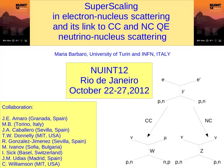
e e' p,n p,n W Z ν µ ν p,n p,n p,n n,p ν CC NC 

Outline

Review of SuperScaling in quasi-elastic inclusive electron scattering Connecting electron and neutrino scattering via SuperScaling: the “SuSA” approach Extended SuSA model: Meson Exchange Currents Application to CC quasielastic neutrino scattering and comparison with MiniBooNE cross sections Application to NC quasielastic neutrino scattering and comparison with MiniBooNE cross sections and ratio p/N Predictions for antineutrino scattering (see Joe Grange's talk for comparison with data)

Many high quality data are available for quasi-elastic electron scattering Any reliable nuclear model must reproduce these data Is there a way to use (e,e') data to predict CC and NC ν-scattering cross sections in the QE region? Answer: yes, exploiting Super-Scaling properties of QE electron scattering

[O. Benhar, D. Day and I. Sick, Rev. Mod. Phys. 80 (2008) , http://faculty.virginia.edu/qes-archive/] [Day,McCarthy,Donnelly,Sick,Ann.Rev.Nucl.Part.Sci.40(1990); Donnelly & Sick, PRC60(1999),PRL82(1999)]

SuperScaling Approximation

Many high quality data are available for quasi-elastic electron scattering Any reliable nuclear model must reproduce these data Is there a way to use (e,e') data to predict CC and NC ν-scattering cross sections in the QE region? Answer: yes, exploiting Super-Scaling properties of QE electron scattering

[O. Benhar, D. Day and I. Sick, Rev. Mod. Phys. 80 (2008) , http://faculty.virginia.edu/qes-archive/] [Day,McCarthy,Donnelly,Sick,Ann.Rev.Nucl.Part.Sci.40(1990); Donnelly & Sick, PRC60(1999),PRL82(1999)]

SuperScaling Approximation

Many high quality data are available for quasi-elastic electron scattering Any reliable nuclear model must reproduce these data Is there a way to use (e,e') data to predict CC and NC ν-scattering cross sections in the QE region? Answer: yes, exploiting Super-Scaling properties of QE electron scattering

[O. Benhar, D. Day and I. Sick, Rev. Mod. Phys. 80 (2008) , http://faculty.virginia.edu/qes-archive/] [Day,McCarthy,Donnelly,Sick,Ann.Rev.Nucl.Part.Sci.40(1990); Donnelly & Sick, PRC60(1999),PRL82(1999)]

yq ,=−pmin

scaling function

Fq, y= d /dd   Mottv LG LvT GT

SuperScaling Approximation

scaling variable (y=0 QEP) Assume that QE scattering is dominated by (e,e'N)

Many high quality data are available for quasi-elastic electron scattering Any reliable nuclear model must reproduce these data Is there a way to use (e,e') data to predict CC and NC ν-scattering cross sections in the QE region? Answer: yes, exploiting Super-Scaling properties of QE electron scattering

[O. Benhar, D. Day and I. Sick, Rev. Mod. Phys. 80 (2008) , http://faculty.virginia.edu/qes-archive/] [Day,McCarthy,Donnelly,Sick,Ann.Rev.Nucl.Part.Sci.40(1990); Donnelly & Sick, PRC60(1999),PRL82(1999)]

Fq , y F  y

q sufficiently large (q>400 MeV/c roughly )

QEP

SuperScaling Approximation

Fq, y= d /dd   Mottv LG LvT GT

scaling function

yq ,=−pmin

Scaling of I kind Assume that QE scattering is dominated by (e,e'N) scaling variable (y=0 QEP)

Many high quality data are available for quasi-elastic electron scattering Any reliable nuclear model must reproduce these data Is there a way to use (e,e') data to predict CC and NC ν-scattering cross sections in the QE region? Answer: yes, exploiting Super-Scaling properties of QE electron scattering

[O. Benhar, D. Day and I. Sick, Rev. Mod. Phys. 80 (2008) , http://faculty.virginia.edu/qes-archive/] [Day,McCarthy,Donnelly,Sick,Ann.Rev.Nucl.Part.Sci.40(1990); Donnelly & Sick, PRC60(1999),PRL82(1999)]

q ,=±T min/T F≃ y/k F

scaling variable (relativistic) scaling function

Fq , F

q large Scaling of I kind

SuperScaling Approximation

Fq ,= d  /d d  Mottv LGLvTGT

Many high quality data are available for quasi-elastic electron scattering Any reliable nuclear model must reproduce these data Is there a way to use (e,e') data to predict CC and NC ν-scattering cross sections in the QE region? Answer: yes, exploiting Super-Scaling properties of QE electron scattering

[O. Benhar, D. Day and I. Sick, Rev. Mod. Phys. 80 (2008) , http://faculty.virginia.edu/qes-archive/] [Day,McCarthy,Donnelly,Sick,Ann.Rev.Nucl.Part.Sci.40(1990); Donnelly & Sick, PRC60(1999),PRL82(1999)]

q large

At ψ>0 scaling is broken by resonances, meson production, etc., mainly in the transverse channel (from analysis of L/T separated data)

Fq , F

Scaling of I kind

SuperScaling Approximation

q ,=±T min/T F≃ y/k F

scaling variable (relativistic)

Fq ,= d  /d d  Mottv LGLvTGT

scaling function

Many high quality data are available for quasi-elastic electron scattering Any reliable nuclear model must reproduce these data Is there a way to use (e,e') data to predict CC and NC ν-scattering cross sections in the QE region? Answer: yes, exploiting Super-Scaling properties of QE electron scattering

[O. Benhar, D. Day and I. Sick, Rev. Mod. Phys. 80 (2008) , http://faculty.virginia.edu/qes-archive/] [Day,McCarthy,Donnelly,Sick,Ann.Rev.Nucl.Part.Sci.40(1990); Donnelly & Sick, PRC60(1999),PRL82(1999)]

f =k F∗F

super-scaling function

k F Fermi momentum

Scaling of II kind super-scaling function

SuperScaling Approximation

Ee=3.6 GeV Θ=16 deg

Plot f as a function of ψ for different nuclei at fixed kinematics:

Many high quality data are available for quasi-elastic electron scattering Any reliable nuclear model must reproduce these data Is there a way to use (e,e') data to predict CC and NC ν-scattering cross sections in the QE region? Answer: yes, exploiting Super-Scaling properties of QE electron scattering

[O. Benhar, D. Day and I. Sick, Rev. Mod. Phys. 80 (2008) , http://faculty.virginia.edu/qes-archive/] [Day,McCarthy,Donnelly,Sick,Ann.Rev.Nucl.Part.Sci.40(1990); Donnelly & Sick, PRC60(1999),PRL82(1999)]

Scaling of II kind Scaling of I kind

SuperScaling Approximation

Ee=3.6 GeV Θ=16 deg

Many high quality data are available for quasi-elastic electron scattering Any reliable nuclear model must reproduce these data Is there a way to use (e,e') data to predict CC and NC ν-scattering cross sections in the QE region? Answer: yes, exploiting Super-Scaling properties of QE electron scattering “SuSA” approach 1) extract the super-scaling function from QE electron scattering data 2) plug it into neutrino cross sections

[O. Benhar, D. Day and I. Sick, Rev. Mod. Phys. 80 (2008) , http://faculty.virginia.edu/qes-archive/] [Day,McCarthy,Donnelly,Sick,Ann.Rev.Nucl.Part.Sci.40(1990); Donnelly & Sick, PRC60(1999),PRL82(1999)]

Rweak ~ Gweak

s.n.* f(ψ)

f(ψ) ~ Rem/Gem

s.n.

SuperScaling Approximation

Formalism: (l,l') inclusive scattering

 l

−

l

−  

W

 −

e,e' e e' ,l

d

2

d ' d' = Mottv L RLvT RT d

2

d ' d' =0V CC RCC2V CL RCLV L L RL LV T RT±2V T ' RT '

2 electromagnetic response functions 5 (3) weak response functions

l=,e ,

Wμν Lμν

Hadronic tensor Leptonic tensor Purely isovector Typically transverse (CC,CL,LL small) Have VV, AA and VA components generated by Jμ=Jμ

V+Jμ A

+ ν – ν

V L RL

CC

L-T-T' separation

MiniBooNE kinematics

,

−

VV-AA-VA separation

MiniBooNE kinematics

,

−

Formalism: (l,l') inclusive scattering



νl

(−)

W

 −

e,e' e e' (ν,ν')

d

2

d ' d' = Mottv L RLvT RT

2 electromagnetic response functions 6 weak response functions

l=,e ,

Wμν Lμν

Hadronic tensor Leptonic tensor NC

d

2σ

d T N d ΩN =σ0[V L R L+V T RT+V TT RTT+V TLRTL±(2V T ' RT '+2V TL' RTL')]

N

ν'l

(−)

t-inclusive t = (ke-k'e)2 u-inclusive u = (kν-pN)2

Phenomenological super-scaling function

The analysis of (e,e') world data shows that:

• 1. Scaling of I kind is reasonably good below the QE peak (ψ<0)
• 2. Scaling of II kind is excellent in the same region
• 3. Scaling violations, particularly of I kind, occur above the QEP and reside mainly in

the transverse response

• 4. The longitudinal response super-scales

A phenomenological super-scaling function has been extracted from the (e,e') world data

[Jourdan, NPA603, 117 ('96)]

L Asymmetric shape: long tail at high energy transfer Only 4 parameters for all kinematics and all nuclei Represents a strong constraint

• n nuclear models

The RFG is very poor: it does super-scale, but to the wrong function!

f RFG=3 4 1−

21− 2

Scaling function(s) and microscopic models

The Relativistic Mean Field

model successfully reproduces the experimental fL

fT

RMF > fL RMF by ~ 20%, in

agreement with exp'tal evidence RPWIA and rROP give a symmetric scaling function and fL=fT

Modified SuSA model: Meson Exchange Currents

MEC are two-body currents involving 2 nucleons exchanging a meson. Currents induced by the pion occur (up to higher order relativistic corrections) in the transverse channel and violate superscaling. We follow a perturbative scheme, considering all the diagrams involving one pion in the two-body current. The calculation is fully relativistic and performed on the basis of RFG.

“contact”

• r

“seagull” “pion-in-flight” “Δ-MEC” Δ π

Meson Exchange Currents: 1p1h and 2p2h many-body diagrams

1p-1h sector:



2p-2h sector

(just a subset of all the 28 many-body

diagrams involving two pionic lines) ⇒ Only contribute inside the RFG response region -1<ψ<1. The net contribution to (e,e') QEP is small due to cancellations between MEC and correlations [Amaro et al., Phys.Rept.368(2002),NPA723 (2003)] Contribute also outside the RFG response region: ψ<-1 and ψ>1

J.W.Van Orden, T.W.Donnelly, Ann. Phys. 131 (1981) Non relativistic calculation with relativistic corrections A.De Pace et al., NPA741 (2004) Fully relativistic calculation

2p-2h MEC in electron scattering

'0 '0

RFG RFG

De Pace et al., NPA741, 249 (2004), RFG-based calculation

Scaling is broken both above and below the QEP 2p-2h MEC give a positive contribution

• f ~10-20% outside the QEP, filling the

“dip” between the QE and ∆ peak.

Inelastic Quasielastic MEC Total

Test of the modified SuSA model: (e,e') cross section

An example:

MEC in “quasielastic” neutrino scattering

In (e,e') experiments Ee is well-known and “QE” means that the electron is scattered by an individual nucleon moving inside the nucleus In (νμ,μ) the neutrino beam is not monochromatic, but it spans a wide range of energies “Flux-averaged” cross section: Each experimental point (θμ,Tμ) takes contribution from different regions in the (q,ω) plane, corresponding to different reaction mechanisms. “QE”=no pions in the final state Processes involving scattering off two or more nucleons must also be considered [Martini et al, Nieves et al]

 d

2

dcosdT  = 1 tot∫ d

2E

dcosdT  EdE

γ e' N' e N

ω=Q2/2mN

〈 E〉=0.788 GeV

MiniBooNE νμ flux

W + ν μ N A μ ν W + ...

QEP

A-2 N1 N2 A A-1

Results for CCQE neutrino scattering

MiniBooNE double differential CCQE cross sections at forward angles

RFG Pauli blocking is active in this region (low momentum transfers, q≲0.4 GeV/c): this explains the big difference between the RFG (where PB is included by definition) and the SuSA (which has no PB) results. At very low angles both RFG and SuSA are compatible with the data, except for the Pauli-blocked region, where super-scaling ideas are not applicable.

MiniBooNE double differential CCQE cross sections at forward angles

MiniBooNE data

RFG Pauli blocking is active in this region (low momentum transfers, q≤0.4 GeV/c): this explains the big difference between the RFG (where PB is included by definition) and the SuSA (which has no PB) results. At very low angles both RFG and SuSA are compatible with the data, except for the Pauli-blocked region, where super-scaling ideas are not applicable. However: about ½ of the cross section for such kinematics arises from the first 50 MeV of excitation, where none of the two approaches should be trusted. Here a proper treatment of collective excitations, like RPA with realistic nuclear wave functions, is required.

[Amaro et al., PLB696 (2011)]

MiniBooNE double differential CCQE cross sections at forward angles

MiniBooNE data

Comparison with MiniBooNE differential CC cross sections

• SuSA predictions fall below the data for

most kinematics

• 2p2h MEC improve the agreement

but are not enough to explain the data

• The effect of 2p2h diagrams decreases

with increasing scattering angle Amaro et al., PLB696 (2011)

Comparison with MiniBooNE differential CC cross sections

• SuSA predictions fall below the data for

most kinematics

• 2p2h MEC improve the agreement

but are not enough to explain the data

• The effect of 2p2h diagrams decreases

with increasing scattering angle Amaro et al., PLB696 (2011)

Strength is missing at lower muon energies and larger scattering angles

Total CC cross section

MB Amaro et al., PLB696 (2011)

FS FSI I

Total CC cross section

MB Amaro et al., PLB696 (2011)

FS FSI I MEC MEC

Total CC cross section

MB Amaro et al., PLB696 (2011)

Results for NCQE neutrino scattering

NC neutrino cross section

Best fit of axial mass at gA

(s)=0

in SuSA and RMF

• R. Gonzalez-Jimenez et al., arXiv:1210.6344

NC p/N ratio: axial strangeness

RMF SuSA Best fits of gA

(s) at fixed MA

The dependence upon the nuclear model is essentially canceled in the ratio gA

(s) = -0.06±0.31 SuSA (χ2/DOF=31.3/29)

gA

(s) = +0.04±0.28 RMF (χ2/DOF=33.6/29)

• R. Gonzalez-Jimenez et al., arXiv:1210.6344

Predictions for antineutrino scattering

CCQE antineutrino cross section

Amaro et al., PRL 208 (2012) The effects of MEC in the present model are found to be very important and significantly larger than for neutrino scattering

NCQE antineutrino cross section

• R. Gonzalez-Jimenez et al., arXiv:1210.6344

Summary

The SuperScaling approach to neutrino scattering: agrees by construction with electron scattering data in a wide range of kinematics; it can be applied to all nuclei (II kind scaling); the superscaling function is phenomenological, but it is well reproduced by the relativistic mean field model. It is based on some assumptions:

• 1. The superscaling function is extracted from longitudinal data and the approach assumes

fL=fT=fT' (true in some, but not all, microscopic models)

• 2. Superscaling violations are not accounted for and must be added (MEC)

Application to the CCQE process leads to cross sections lower than the MiniBooNE data Addition of 2p2h MEC diagrams improves the agreement but still misses the data at higher scattering angles and lower muon energies (however, the axial MEC are missing) Application to the NCQE process gives results lower than the MiniBooNE data at low Q2 (but no MEC in the present model) Improvements of the model (in progress):

• 1. Inclusion of axial MEC in the 2p2h sector
• 2. Inclusion of correlations associated to MEC, necessary to preserve gauge invariance

Backup Slides

Relativistic effects

• 1. Relativistic Kinematics: Ep=m+p2/(2m) Ep=√p2+m2
• 2. Relativistic Current Operators: Dirac spinors and γ -matrices
• 3. Relativistic treatment of the nuclear dynamics

All these effects are large at the typical neutrino energies of current experiments (Eν∼ 1-few GeV) Reliable nuclear modeling in the 1 GeV region cannot neglect relativistic effects

= Q

2

2m = q

2

2m

Expressions for the π-exchange currents

J 2

 =J s  J   J  

“Seagull”:

J s

 p' 1, p' 2; p1, p2= f 2

m

2 i3abup' 1a5 K1u p1

F1

V

K1

2−m 2 u p' 2b5 up21⇔2

“Pion-in-flight”:

J 

  p' 1, p' 2; p1, p2= f 2

m

2 i 3abu p'1a5  K1u p1

FK1−K2



K 1

2−m 2K 2 2−m 2  u p'2b5  K2up2

“Δ-MEC”:

J 

  p' 1, p' 2; p1, p2=f N f

m

2

u p'1T a

15u p11

K 2

2−m 2 u p'2a5  K 2u p21⇔2

T a

1=K2 G   H 1Q S f  H 1T aT 3T 3T aSb  P' 1G   P' 1−Q  K2



 =g − 1

4 

 

Rarita-Schwinger propagator Forward and backward Δ-electroexcitation tensors

Correlation Currents

In order to preserve gauge invariance correlation diagrams, where the virtual boson attaches to one of two interacting nucleons, must be also considered:

N

The total two-body current is conserved:

∂ μ J(2)

μ = 0

Correlation currents contribute to both longitudinal and transverse channels.

Relativistic Impulse Approximation Models

RIA: Scattering off a nucleus ⇒Incoherent sum of single-nucleon scattering processes Nuclear current ⇒ One-body operator

1) Relativistic Mean Field Model - RMF 2) Semi-relativistic Shell Model - RSM 4) Relativistic Green's Function - RGF In the RMF approach

ΨB: bound nucleon w.f. ⇒ Relativistic Mean Field (strong S and V potentials) ΨF: ejected nucleon w.f. ⇒ Final State Interaction, treated in different approaches: RPWIA: relativistic plane wave (no FSI) rROP: real relativistic optical potential RMF: uses the same RMF employed for the initial state

J N

 ,q=∫d 

pF p qJ N

 B

p

Relativistic Fermi Gas and super-scaling

The nucleus is a collection of free nucleons described by Dirac spinors u(p,s) The only correlations between nucleons are the Pauli correlations Lorentz covariance and Gauge invariance exactly fulfilled Response functions: R K,=GK ,f RFG

=  2mN ,= q 2mN ,=

2− 2

dimensionless variables single-nucleon functions “super-scaling” function (universal)

,= 1

F

−

11

RFG scaling variable

F Fermi kinetic energy

kF Fermimomentum Es energy shift typically~20 MeV : '=−Es '=' ,' f RFG= 3 4 1−

21− 2

Two parameters: fixed by fitting the position and the width of the QEP.

The RFG predicts that if the nuclear cross section is divided by the single nucleon one and plotted versus ψ for different values of the momentum transfer q and kF, the result is 1) independent of q: scaling of first kind 2) independent of kF: scaling of second kind

=0QEP

parabola The RFG exactly super-scales All scaling functions (L,T,T') are equal

Scaling in the Delta region

[

d

2

d d ]' ' =[ d

2

d d ]exp −[ d

2

d d ]QE

1) subtract the QE contribution obtained from Superscaling hypothesis 2) divide by the elementary N →∆ cross section

F' '=

[

d

2

dd ]' '  MvLGL

vT GT 

3) multiply by the Fermi momentum

f ' '=kF F' '

4) plot versus the appropriate scaling variable

=q , =1 1 4 m

2 /mN 2 −1

inelasticity

Ee=0.3−4GeV =12−145

12 C, 16O

This approach can work only at Ψ∆<0, since at ΨΔ>0 other resonances and the tail of DIS contribute

Amaro, Barbaro, Caballero, Donnelly, Molinari, Sick, PRC71 (2005)