Math 5490 11/3/2014 Dynamical Systems Math 5490 Summary So Far - - PDF document

SLIDE 1

Math 5490 11/3/2014 Richard McGehee, University of Minnesota 1

Topics in Applied Mathematics: Introduction to the Mathematics of Climate

Mondays and Wednesdays 2:30 – 3:45

http://www.math.umn.edu/~mcgehee/teaching/Math5490-2014-2Fall/

Streaming video is available at

http://www.ima.umn.edu/videos/

Click on the link: "Live Streaming from 305 Lind Hall". Participation:

https://umconnect.umn.edu/mathclimate

Math 5490

November 3, 2014

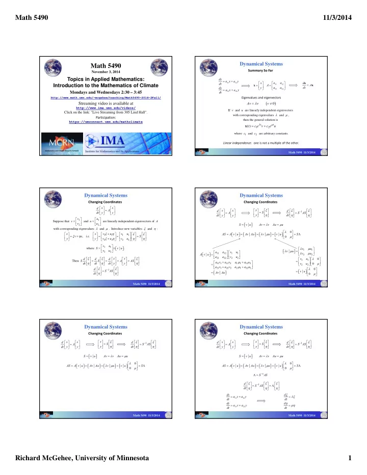
Dynamical Systems

11 12 21 22

dx a x a y dt dy a x a y dt     Math 5490 11/3/2014

11 12 21 22

a a x A a a y               x d A dt  x x

Summary So Far

Eigenvalues and eigenvectors If and are linearly independent eigenvectors with corresponding eigenvalues and , then the general solution is v u  

1 2

( )

t t

t c e v c e u

 

  x

1 2

where and are arbitrary constants. c c

 

Av v v   

Linear independence: one is not a multiple of the other.

Dynamical Systems

Math 5490 11/3/2014 x x d A y y dt             

Changing Coordinates

1 1 2 2

Suppose that and are linearly independent eigenvectors of with corresponding eigenvalues and . Introduce new variables and : , i.e. v u v u A v u v x x v u y y                                   

1 1 1 1 2 2 2 2

u v u S v u v u                                    

1 1 2 2

where = . v u S v u v u           

1

Then x x d d d S S A AS y y dt dt dt d S AS dt          



                                              

Dynamical Systems

Math 5490 11/3/2014 x x d A y y dt             

Changing Coordinates

x S y                S v u Av v Au u         

1

d S AS dt    



             AS A v u Av Au v u v u S                                

11 12 1 1 21 22 2 2 11 1 12 2 11 1 12 2 21 1 22 2 21 1 22 2

a a v u A v u a a v u a v a v a u a u a v a v a u a u Av Au                                 

1 1 2 2 1 1 2 2

v u v u v u v u v u v u                                             

Dynamical Systems

Math 5490 11/3/2014 x x d A y y dt             

Changing Coordinates

x S y                S v u Av v Au u         

1

d S AS dt    



             AS A v u Av Au v u v u S                                

Dynamical Systems

Math 5490 11/3/2014 x x d A y y dt             

Changing Coordinates

x S y                S v u Av v Au u         

1

d S AS dt    



             AS A v u Av Au v u v u S                                

1

S AS



 

1

d S AS dt      



                    

11 12 21 22

dx a x a y dt dy a x a y dt     d dt d dt      

SLIDE 2

Math 5490 11/3/2014 Richard McGehee, University of Minnesota 2

Dynamical Systems

eigenvalues: 2 and 1 2 1 eigenvectors: and . 1 1               Example 2 dx x y dt dy x dt    2 1          1 2 1 A        Math 5490 11/3/2014

Changing Coordinates

2 1 1 1 S         2 x y         2 1 2 1 1 x S y                                             2 dx x y dt dy x dt    2 x y         2 d dt d dt       

Dynamical Systems

Example dx y dt dy x dt    i i          1 1 A        

Math 5490 11/3/2014

Changing Coordinates

1 1 i i S         x iz iw y z w     1 1 x z i i z iz iw S y w w z w                                     dx y dt dy x dt    dz iz dt dw iw dt    eigenvalues: eigenvectors: 1 1 i i i i               x iz iw y z w    

Dynamical Systems

Example

Math 5490 11/3/2014

Changing Coordinates

dx y dt dy x dt    dz iz dt dw iw dt    x iz iw y z w     Note that one of these equations is redundant. 2 2 z y ix w z w y ix       dz iz dt  1 dr dt d dt    dx y dt dy x dt    Cartesian complex polar

Dynamical Systems

Example dx ax y dt dy x ay dt       x a x x d A y a y y dt                              a A a          

2 2

trace( ) 2 det( ) A a a a A a          

2 2 2 2

det( ) 2 A I a a              

2 2 2 2

4 2 4 4 4 The eigenvalues are 2 2 and a a a a i a i a i                   

Changing Coordinates

Math 5490 11/3/2014

Dynamical Systems

Let . z x iy  

( ) ( ) ( )

Solution: ( )

i i t a i t a i t at

z t z e r e e r e e

       

   ( ) dz a i z dt    Let .

i

z re   dr ar dt d dt     ( ) Solution: ( )

at

r t r e t t       dx ax y dt dy x ay dt       Then ( )( ) dz dx dy i dt dt dt ax y i x iay a i x iy             Then ( ) ( ) ( )

i i i

dz dr d e rie a i z a i re dt dt dt dr d ri a i r dt dt

  

             

Changing Coordinates

Math 5490 11/3/2014

Dynamical Systems

If is a matrix with real elements and if is an eigenvalue of with corrresponding eigenvector , then is an eigenvalue of with corresponding eigenvector . A A v A v   Complex Eigenvalues

Math 5490 11/3/2014

Av v Av v Av v        

SLIDE 3

Math 5490 11/3/2014 Richard McGehee, University of Minnesota 3

Dynamical Systems

dx Ax dt 

Spirals

Math 5490 11/3/2014 1 1 A         2 1 1 2 A           2 1 1 2 A          

x x x y y y center stable spirals

dz iz dt  ( 2 ) dz i z dt    ( 2 ) dz i z dt    ( ) ( ) r t r t t     

2

( ) ( )

t

r t r e t t  



  

2

( ) ( )

t

r t r e t t  



  

x x x y y y

Dynamical Systems

dx Ax dt 

Spirals

Math 5490 11/3/2014 1 1 A         2 1 1 2 A         2 1 1 2 A        

center unstable spirals

dz iz dt   (2 ) dz i z dt   (2 ) dz i z dt   ( ) ( ) r t r t t     

2

( ) ( )

t

r t r e t t     

2

( ) ( )

t

r t r e t t     

Dynamical Systems

Example 4 2 5 dx x y dt dy x y dt      4 2 1 5 x x x d A y y y dt                             4 3 2 1 2 3 1 5 3 1 2 2 3 1 A I v                                trace( ) 4 5 9 det( ) ( 4) ( 5) 2 1 18 A A                

2 2

det( ) 9 18 ( 3)( 6) A I                   The eigenvalues are 3 and 6.      

Changing Coordinates

Math 5490 11/3/2014 4 2 1 5 A          4 6 2 2 2 6 1 5 6 1 1 1 6 1 A I v                              

1

2 1 3 1 1 6 S S AS S AS



                     

Dynamical Systems

Example 4 2 5 dx x y dt dy x y dt     

Changing Coordinates

Math 5490 11/3/2014 2 1 1 1 x y                       3 6 d dt d dt        

η ξ y x

Dynamical Systems

Example 3 4 2 3 dx x y dt dy x y dt       3 4 2 3 x x x d A y y y dt                             3 1 4 2 4 2 3 1 2 4 2 1 1 A I v                                trace( ) 3 3 det( ) ( 3) 3 4 ( 2) 1 A A                

2 2

det( ) 1 ( 1)( 1) A I                 The eigenvalues are 1 and 1.     

Changing Coordinates

Math 5490 11/3/2014 3 4 2 3 A          3 1 4 4 4 2 3 1 2 2 1 1 1 A I v                              

1

2 1 1 1 1 1 S S AS S AS



                   

Dynamical Systems

Example 3 4 2 3 dx x y dt dy x y dt      

Changing Coordinates

Math 5490 11/3/2014 2 1 1 1 x y                      d dt d dt       

η ξ y x

SLIDE 4

Math 5490 11/3/2014 Richard McGehee, University of Minnesota 4

Dynamical Systems

11 12 21 22

dx a x a y dt dy a x a y dt     Math 5490 11/3/2014

11 12 21 22

a a x A a a y               x d A dt  x x

Summary

Suppose that and are linearly independent eigenvectors of with corresponding eigenvalues and . Introduce new variables and : , where . Then v u A x S S v u y                              

1

, and the system becomes S AS



     d dt d dt      

Dynamical Systems

Math 5490 11/3/2014 x x d A y y dt             

Eigenvalues

2 2 1 2 2 1 2 1 2

det( ) trace( ) det( ) ( )( ) ( ) A I A A                              

1 2 1 2

trace( ) det( ) A A       

The trace is the sum of the eigenvalues, while the determinant is the product of the eigenvalues. We can characterize the dynamic behavior using the trace and the determinant

Dynamical Systems

Math 5490 11/3/2014 x x d A y y dt             

Saddles

1 2

det( ) A    

y x

‐2 ‐1 1 2 ‐2 ‐1 1 2 ‐2 ‐1 1 2 ‐2 ‐1 1 2

One eigenvalue is positive, the other negative. trace/2 determinant

2

trace det    

‐2 ‐1 1 2 ‐2 ‐1 1 2

Dynamical Systems

Math 5490 11/3/2014 x x d A y y dt             

Stable Nodes

1 2 1 2

det( ) trace( ) A A              Both eigenvalues are negative. trace/2 determinant

2 2

4 2             

y x

2

discriminant 4     

‐2 ‐1 1 2 ‐2 ‐1 1 2

Dynamical Systems

Math 5490 11/3/2014 x x d A y y dt             

Stable Spirals

Both eigenvalues are complex, with negative real part. determinant

x y

1 2 1 2

det( ) trace( ) A A              trace/2

2 2

4 2 i             

2

4    

‐2 ‐1 1 2 ‐2 ‐1 1 2

Dynamical Systems

Math 5490 11/3/2014 x x d A y y dt             

Unstable Nodes

Both eigenvalues are positive. determinant

y x

1 2 1 2

det( ) trace( ) A A              trace/2

2 2

4 2             

2

4    

SLIDE 5

Math 5490 11/3/2014 Richard McGehee, University of Minnesota 5

‐2 ‐1 1 2 ‐2 ‐1 1 2

Dynamical Systems

Math 5490 11/3/2014 x x d A y y dt             

Unstable Spirals

Both eigenvalues are complex, with positive real part. determinant

1 2 1 2

det( ) trace( ) A A              trace/2

2 2

4 2 i             

2

4    

x y

Dynamical Systems

Math 5490 11/3/2014

Classification

Kaper & Engler, 2013 determinant trace

Dynamical Systems

Math 5490 11/3/2014

Degenerate Cases

1 2

det( ) A     One of the eigenvalues is zero, the other positive. dx x dt dy dt   rest points Kaper & Engler, 2013

Dynamical Systems

Math 5490 11/3/2014

Degenerate Cases

1 2

det( ) A     One of the eigenvalues is zero, the other negative. dx x dt dy dt    rest points Kaper & Engler, 2013

Dynamical Systems

Math 5490 11/3/2014

Degenerate Cases

1 2 1 2

trace( ) det( ) A A          Both eigenvalues are imaginary. dx y dt dy x dt   

x y

center Kaper & Engler, 2013

Dynamical Systems

Math 5490 11/3/2014

Degenerate Cases

Positive double eigenvalue. Only one eigenvector dx x y dt dy y dt   

degenerate node

1 2 1 2

det( ) trace( ) A A             

2

4     Kaper & Engler, 2013

SLIDE 6

Math 5490 11/3/2014 Richard McGehee, University of Minnesota 6

Dynamical Systems

Math 5490 11/3/2014

Degenerate Cases

Negative double eigenvalue. Only one eigenvector dx x y dt dy y dt     

degenerate node

1 2 1 2

det( ) trace( ) A A             

2

4     Kaper & Engler, 2013

Dynamical Systems

Math 5490 11/3/2014

Topological Classification

If neither eigenvalue has zero real part, then the system is called hyperbolic, in which case, there are only three classes:

• 1. saddles: One positive eigenvalue and one negative. The determinant

is negative.

• 2. sources: Both eigenvalues have positive real part. The determinant is

positive, and the trace is positive.

• 3. sinks: Both eigenvalues have negative real part. The determinant is

positive, and the trace is negative. Every system in one of the three categories looks the same to a topologist (topological conjugacy).