Methods of proof for residuated algebras of binary relations - - PowerPoint PPT Presentation

Methods of proof for residuated algebras

• f binary relations

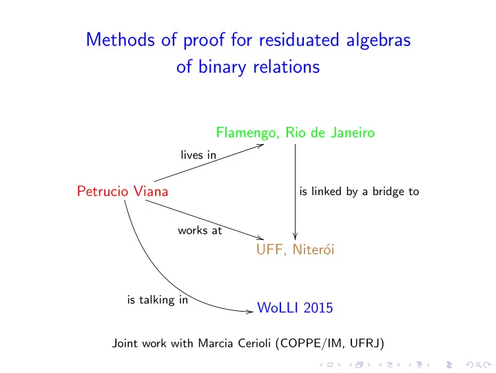
Flamengo, Rio de Janeiro

is linked by a bridge to

• Petrucio Viana

lives in

• works at
• is talking in
• UFF, Niter´
• i

WoLLI 2015

Joint work with Marcia Cerioli (COPPE/IM, UFRJ)

Outline

• 1. Binary relations and some of their operations
• 2. Residuated algebras of binary relations
• 3. Algebraic and quasi-algebraic theories of residuated algebras
• f binary relations
• 4. Calculational reasoning
• 5. Diagrammatic reasoning
• 6. Perspectives

• 1. Binary relations and some of their operations

Binary relations

Let U be a set. Elements of U are usually denoted by u, v, w, . . . A binary relation on U is a subset of U × U. 2RelU is the set of all binary relations on U. Elements of 2RelU are usually denoted by R, S, T, . . .

Operations on binary relations

Let R, S ∈ 2RelU. Booleans The union of R and S is: R ∪ S = {(u, v) ∈ U : (u, v) ∈ R or (u, v) ∈ S} The intersection of R and S is: R ∪ S = {(u, v) ∈ U : (u, v) ∈ R and (u, v) ∈ S}

Operations on binary relations

Let R, S ∈ 2RelU. Peirceans The composition of R and S is: R ◦ S = {(u, v) ∈ U : ∃w ∈ U[(u, w) ∈ R and (w, v) ∈ S]} The reversion of R is: R−1 = {(u, v) ∈ U : (v, u) ∈ R}

Operations on binary relations

Let R, S ∈ 2RelU. Between Booleans and Peirceans The left residuation of R and S is: R\S = {(u, v) ∈ U : ∀w ∈ U[ if (w, u) ∈ R, then (w, v) ∈ S]} The right residuation of R and S is: R/S = {(u, v) ∈ U : ∀w ∈ U[ if (v, w) ∈ S, then (u, w) ∈ R]}

Motivations for residuals

– Algebra: M. Ward and R.P. Dilworth. Residuated lattices.

• Trans. Amer. Math. Soc. 45: 335–54 (1939)

– Computer Science: C.A.R Hoare and H. Jifeng. The weakest

• prespecification. Fund. Inform. 9: Part I 51–84, Part II

217–252 (1986) – Linguistics: J. Lambek. The mathematics of sentence

• structure. Amer. Math. Monthly 65: 154–170 (1958)

– Logic: N. Galatos, P. Jipsen, T. Kowalski, and H. Ono . Residuated Lattices. An Algebraic Glimpse at Substructural

• Logics. Elsevier (2007)

• 2. Residuated algebras of binary relations

Residuated algebras of relations

Let U be a set. Let A ⊆ 2RelU be closed under all the operations ∪, ∩, ◦, −1, \ and /. The residuated algebra of binary relations on U based on A is the algebra: A = A, ∪, ∩, ◦, −1, \, / A2Rel is the class of all residuated algebra of binary relations. Elements of A2Rel are usually denoted by A, B, C, . . .

Residuated algebras of relations

Aka lattice-ordered involuted residuated semigroups:

• 1. Lattice: R ∪ S is a supremum and R ∩ S is a infimum.
• 2. Ordered: R ≤ S (iff R ∪ S = S iff R ∩ S = R) is a parcial
• rdering.
• 3. Semigroup: R ◦ S is a not necessarily commutative

multiplication.

• 4. Involuted: (R−1)−1 = R and (R ◦ S)−1 = S−1 ◦ R−1.
• 5. Residuated: \ is the left-inverse of ◦ and / is the right inverse
• f ◦.

• 3. Algebraic and quasi-algebraic theories of

residuated algebras of binary relations

Terms and inclusions

The terms, typically denoted by R, S, T, . . ., are generated by: R ::= X | R ∪ R | R ∩ S | R ◦ R | R\R | R/R | R−1 where X ∈ Var, a set of variables fixed in advance. A quasi-equality is an expression of the form R ⊆ S where R and S ate terms.

Horn quasi-equalities

A Horn quasi-equality is an expression of the form R1 ⊆ S1, . . . , Rn ⊆ Sn ⇒ R ⊆ S where R1, S2, . . . , Rn, Sn, R, S are terms.

Valuations and values

Let A ∈ A2Rel. A valuation on A is a function v : Var → A. Let R be a term, A ∈ A2Rel, and v be a valuation on A. The value of R in A according to v, denoted by RA

v is defined by:

X A

v

= vX (R ∪ S)A

v

= RA

v ∪ SA v

(R ∩ S)A

v

= RA

v ∩ SA v

(R ◦ S)A

v

= RA

v ◦ SA v

(R\S)A

v

= RA

v \SA v

(R−1)A

v

= (RA

v )−1

Truth and validity

Let R ⊆ S be a quasi-equality, A ∈ A2Rel, and v be a valuation

• n A.

R ⊆ S is true on A under v if RA

v ⊆ SA v .

R ⊆ S is identically true on A, or A is a model of R ⊆ S, if R ⊆ S is true on A under v, for every valuation v. R ⊆ S is valid if every residuated algebra of relations A is a model

• f R ⊆ S.

Validity and consequence

Let R1 ⊆ S1, . . . , Rn ⊆ Sn ⇒ R ⊆ S (1) be a Horn quasi-equality, A ∈ A2Rels, and v be a valuation on A. (1) is valid, or R ⊆ S is a consequence of R1 ⊆ S1, . . . , Rn ⊆ Sn, if every model of all R1 ⊆ S1, . . . , Rn ⊆ Sn is a model of R ⊆ S.

From quasi-equalities to equalities and back

An equality is an expression of the form R = S where R and S ate terms. A Horn equality is an expression of the form R1 = S1, . . . , Rn = Sn ⇒ R = S where R1, S2, . . . , Rn, Sn, R, S are terms.

From quasi-equalities to equalities and back

True, identically true, and valid equalities are defined as usual.

From quasi-equalities to equalities and back

Since R ⊆ S is valid iff R ∩ S ⊆ S and S ⊆ R ∩ S are both valid, we can consider to build the algebraic and the quasi-algebraic theories of the residuated algebras of relations on the top of the logic of equality. But, taking equational logic as the subjacent logic, we have the following . . .

Negative results

The set of all valid equalities (quasi-equalities) is not finitely axiomatizable (Mikul´ as, IGPL, 2010). The set of all valid Horn equalities (Horn quasi-equalities) is not finitely axiomatizable (Andr´ eka and Mikul´ as, JoLLI, 1994).

Negative results

One proper question is: are there interesting alternatives for equational reasoning on residuated algebras of binary relations?

• 4. Calculational reasoning

Quasi-posets

Let P be a set and R be a binary relation on P. P, R is a quasi-poset if R is reflexive and transitive (but not necessarily antisymmetric) on P.

Galois connections

Let P1 = P1, ≤1, P2 = P2, ≤2 be quasi-posets, and f : P1 → P2, g : P2 → P1 be functions. P1, P2, f , g is a Galois connection if, for all x ∈ P1 and y ∈ P2: fx ≤2 y ⇐ ⇒ x ≤1 gy

Calculational rules

Quasi-poset rules ⊤ x ≤ x

Ref

x ≤ y . . . y ≤ z x ≤ z

Tra

GC rules fx ≤ y x ≤ gy

GC

x ≤ gy fx ≤ y

GC

These rules aloud us to perform both direct and indirect calculational reasoning (without negation).

Direct calculational proofs

A direct calculational proof of t1 ≤ t2 is a sequence t1 ≤ t2, t3 ≤ t4, . . . , tn−1 ≤ tn such that, for each i, 3 ≤ i ≤ n, ti ≤ ti+1, at least one oh the following conditions hold:

• 1. ti ≤ ti+1 is an axiom.
• 2. ti ≤ ti+1 is obtained from previou(s) quasi-equation(s) in the

sequence by one application of some calculational rule.

• 3. tn−1 ≤ tn is an axiom.

Start with t1 ≤ t2 and applying axioms and calculational rules arrive in an axiom.

Direct calculational proofs from hypothesis

Let Γ be a set of quasi-equations. A direct calculational proof of t1 ≤ t2 from Γ is a sequence t1 ≤ t2, t3 ≤ t4, . . . , tn−1 ≤ tn such that, for each ti ≤ ti+1, where 3 ≤ i ≤ n, at least one of the following conditions hold:

• 1. ti ≤ ti+1 is an axiom
• 2. ti ≤ ti+1 ∈ Γ
• 3. ti ≤ ti+1 is obtained from previou(s) quasi-equation(s) in the

sequence by one application of some Calculational Rule.

• 4. tn−1 ≤ tn is an axiom or belongs to Γ.

Start with t1 ≤ t2 and applying axioms, hyphotesis, and calculational rules arrive in an axiom or hyphotesis.

∪ defines a Galois connection

Let A, ⊆ ∈ A2Rel and take A × A, ⊆ × ⊆ ∈ A2Rel. For all X, Y ∈ A, we define f : A × A → A by: f (X, Y ) = X ∪ Y and g : A → A × A by: g(X) = (X, X) With these notations, for all R, S, T ∈ A: R ∪ S ⊆ T ⇐ ⇒ R ⊆ T and S ⊆ T is the same as f (R, S) ⊆ T ⇔ (R, S) ⊆ g(T)

\ defines a family of Galois connections

Let A, ⊆ ∈ A2Rel. For every R ∈ A, we define: fR(X) = R ◦ X and gR(X) = R\X With these notations, we have that R ◦ S ⊆ T ⇔ S ⊆ R\T is the same as fR(S) ⊆ T ⇔ S ⊆ gR(T)

∩, −1 and / define Galois connections

Sorry, no time to enter in details!

Basic arithmetical results

T1) S ⊆ R\(R ◦ S) S ⊆ R\(R ◦ S) GC R ◦ S ⊆ R ◦ S Ref ⊤

Basic arithmetical results

T2) R ◦ (R\S) ⊆ S R ◦ (R\S) ⊆ S GC R\S ⊆ R\S Ref ⊤

Basic arithmetical results

T3) R\(S ∩ T) ⊆ (R\S) ∩ (R\T) R\(S ∩ T)] ⊆ (R\S) ∩ (R\T) GC R\(S ∩ T)] ⊆ R\S ∧ R\(S ∩ T) ⊆ S\T GC R ◦ [R\(S ∩ T)] ⊆ S ∧ R ◦ [R\(S ∩ T)] ⊆ T GC R ◦ [R\(S ∩ T)] ⊆ S ∩ T GC R\(S ∩ T) ⊆ R ◦ (S ∩ T) Ref ⊤

Basic arithmetical results

T4) S ⊆ T = ⇒ R\S ⊆ R\T S ⊆ T T2 R ◦ (R\S) ⊆ T GC R\S ⊆ R\T By T2, R ◦ (R\S) ⊆ S.

Basic arithmetical results

T5) T1, T2, T3 = ⇒ GC for \ R ◦ S ⊆ T ⇓ Mon, Ide R ◦ S ⊆ (R ◦ S) ∩ T ⇓ T4 R\(R ◦ S) ⊆ R\[(R ◦ S) ∩ T] ⇓ T1 S ⊆ R\[(R ◦ S) ∩ T] ⇓ T3 S ⊆ R\T By T1, S ⊆ R\(R ◦ S). By T3, R\[(R ◦ S) ∩ T] ⊆ R\T.

Basic arithmetical results

T5) T1, T2, T3 = ⇒ GC for \ S ⊆ R\T ⇓ Mon R ◦ S ⊆ R ◦ (R\T) ⇓ T2 R ◦ S ⊆ T By T2, R ◦ (R\S) ⊆ S

Indirect calculational proofs

An indirect calculational proof of t1 ≤ tn is a sequence x ≤ t1, t2 ≤ t3, . . . , x ≤ tn such that ti ≤ ti+1 —for each i, 2 ≤ i ≤ n − 1— and x ≤ tn are

• btained from previou(s) quasi-equation(s) in the sequence by one

application of some calculational rule. Suppose x ≤ t1 and prove x ≤ t2 by applying the calculational rules.

Indirect calculational proofs from hyphotesis

Let Γ be a set of quasi-equations. A direct calculational proof of t1 ≤ tn from Γ is a sequence x ≤ t1, t2 ≤ t3, . . . , x ≤ tn such that, for each ti ≤ ti+1, where 2 ≤ i ≤ n − 1, at least one of the following conditions hold:

• 1. ti ≤ ti+1 is an axiom
• 2. ti ≤ ti+1 ∈ Γ
• 3. ti ≤ ti+1 is obtained from previou(s) quasi-equation(s) in the

sequence by one application of some calculational rule.

• 4. x ≤ tn is an axiom or belongs to Γ.

Suppose x ≤ t1 and prove x ≤ t2 by applying axioms, hyphotesis, and calculational rules.

Basic arithmetical results

T6) (R\S) ∩ (R\T) ⊆ R\(S ∩ T) X ⊆ (R\S) ∩ (R\T) GC X ⊆ R\S ∧ X ⊆ R\T GC R ◦ X ⊆ S ∧ R ◦ X ⊆ T GC R ◦ X ⊆ S ∩ T GC X ⊆ R\(S ∩ T) Hence, (R\S) ∩ (R\T) ⊆ R\(S ∩ T) and R\(S ∩ T) ⊆ (R\S) ∩ (R\T) (this is a bonus!).

Some questions

To determine the strengths of: (1) direct calculational proofs, (2) direct calculational proofs from hypothesis, (3) indirect calculational proofs, and (4) indirect calculational proofs from hyphotesis.

• 5. Diagrammatic reasoning

Digraphs

A directed labelled multi graph is a structure N, A, where:

• 1. N is a set of nodes
• 2. A ⊆ N × Terms × N is a set of arcs labeled by terms

Nodes are usually denoted by u, v, w, . . . Digraphs are usualy denoted by G, H, I, . . .

Homomorphisms

Let G1 = N1, A1 and G2 = N2, A2 be digraphs. A homomorphism from G1 to G2 is a mapping h : N1 → N2 such that: (hu, t, hv) ∈ A2 whenever (u, t, v) ∈ A1 A mapping that preserves labels.

2-pointed graphs

A 2-pointed digraph is a structure N, A, s, t, where:

• 1. N, A is the subjacent digraph
• 2. s, t ∈ N, where s is the source and t is the target

2-pointed digraphs are usually denoted by G, s, t.

2-pointed Homomorphisms

Let G1 = N1, A1, s1, t1 and G2 = N2, A2, s2, t2 be 2-pointed digraphs. A 2-pointed homomorphism from G1 to G2 is a homomorphism h : N1 → N2 such that: hs1 = s2 and ht1 = t2 A homomorphism that preserves source and target.

Operations on diagrams

Split digraphs

• R∪S

=

• R
• | •

S

Paralelize arcs

• R∩S

=

• R
• S

Operations on diagrams

Sequentialize arcs

• R◦S

=

• R

S

Revert arcs

• R−1

=

• R

Operations on diagrams

Close digraphs

• R

R\S

⊆

• R
• S
• R\S

Add residuals

• S

⊆

• S
• R\(R◦S)

Operations on diagrams

Hyphotesis rule R ⊆ S ∧

• R

⊆

• R
• S

Hybrid rule S ⊆ T ∧

• R\S •

⊆

• R\T •

Basic arithmetical results

Suppose R ◦ S ⊆ T. We shall prove S ⊆ R\T by means of diagrams.

Basic arithmetical results

Start with the graph of the left hand side: −

S

+

Basic arithmetical results

Apply add residuals: −

S

• R\(R◦S)

+

Basic arithmetical results

Apply hybrid rule, together with the hyphotesis R ◦ S ⊆ T: −

S

• R\T

+

Basic arithmetical results

Apply homomorphism, erasing superfluous arcs: −

R\T

+

Basic arithmetical results

Suppose S ⊆ R\T. We shall prove R ◦ S ⊆ T by means of diagrams.

Basic arithmetical results

Start with the graph of the left hand side: −

R◦S

+

Basic arithmetical results

Apply sequencialize arcs: −

R

S

+

Basic arithmetical results

Apply the hyphotesis R ⊆ R\T: −

R

S

• R\T

+

Basic arithmetical results

Apply close diagram: −

R

• T
• S
• R\T

+

Basic arithmetical results

Apply homomorphism, arasing superfluous arcs: −

T

+

Some questions

(1) To determine the strengths of the proofs with graphs. (2) To compare equational reasoning with calculational reasoning with diagrammatic reasoning.