Moore s Law s Law Moore Super Scalar/Vector/Parallel 1 PFlop/s - - PDF document

moore s law s law moore
SMART_READER_LITE
LIVE PREVIEW

Moore s Law s Law Moore Super Scalar/Vector/Parallel 1 PFlop/s - - PDF document

Self- -Adapting Adapting Self Numerical Software Numerical Software (SANS- -Effort) Effort) (SANS Jack Dongarra, Innovative Computing Laboratory University of Tennessee and Computer Science and Mathematics Division Oak Ridge National


slide-1
SLIDE 1

1

Self Self-

  • Adapting

Adapting Numerical Software Numerical Software (SANS (SANS-

  • Effort)

Effort)

Jack Dongarra,

Innovative Computing Laboratory University of Tennessee and Computer Science and Mathematics Division Oak Ridge National Laboratory

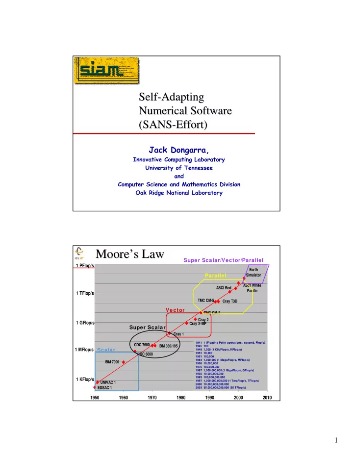
Earth Simulator ASCI White Pacific EDSAC 1 UNIVAC 1 IBM 7090 CDC 6600 IBM 360/195 CDC 7600 Cray 1 Cray X-MP Cray 2 TMC CM-2 TMC CM-5 Cray T3D ASCI Red

1950 1960 1970 1980 1990 2000 2010 1 KFlop/s 1 MFlop/s 1 GFlop/s 1 TFlop/s 1 PFlop/s

Scalar Super Scalar Vector Parallel Super Scalar/Vector/Parallel

Moore Moore’ ’s Law s Law

1941 1 (Floating Point operations / second, Flop/s) 1945 100 1949 1,000 (1 KiloFlop/s, KFlop/s) 1951 10,000 1961 100,000 1964 1,000,000 (1 MegaFlop/s, MFlop/s) 1968 10,000,000 1975 100,000,000 1987 1,000,000,000 (1 GigaFlop/s, GFlop/s) 1992 10,000,000,000 1993 100,000,000,000 1997 1,000,000,000,000 (1 TeraFlop/s, TFlop/s) 2000 10,000,000,000,000 2003 35,000,000,000,000 (35 TFlop/s)

slide-2
SLIDE 2

2

Linpack (100x100) Analysis Linpack (100x100) Analysis

♦ Compaq 386/SX20 SX with FPA - .16 Mflop/s ♦ Pentium IV – 2.8 GHz – 1.32 Gflop/s ♦ 12 years we see a factor of ~ 8231 ♦ Moore’s Law says something about a factor of 2

every 18 months or a factor of 256 over 12 years

♦ Where is the missing factor of 32 …

Clock speed increase = 128x External Bus Width & Caching –

16 vs. 64 bits = 4x

Floating Point -

4/8 bits multi vs. 64 bits (1 clock) = 8x

Compiler Technology = 2x

♦ However the theoretical peak for that Pentium 4

is 5.6 Gflop/s and here we are getting 1.32 Gflop/s

Still a factor of 4.25 off of peak

Complex set of interaction between Users’ applications Algorithm Programming language Compiler Machine instruction Hardware Many layers of translation from the application to the hardware Changing with each generation

Where Does the Performance Go? or Where Does the Performance Go? or Why Should I Care About the Memory Hierarchy? Why Should I Care About the Memory Hierarchy?

1 100 10000 1000000 1 9 8 1 9 8 2 1 9 8 4 1 9 8 6 1 9 8 8 1 9 9 1 9 9 2 1 9 9 4 1 9 9 6 1 9 9 8 2 2 2 2 4

Year Performance

Processor-DRAM Memory Gap (latency) µProc 60%/yr. (2X/1.5yr) DRAM 9%/yr. (2X/10 yrs) “Moore’s Law” Processor-Memory Performance Gap: (grows 50% / year)

CPU DRAM

slide-3
SLIDE 3

3

The Memory Hierarchy The Memory Hierarchy

Registers Level 1 Cache 1cy 3-10 words/cycle compiler managed 1-3cy 1-2 words/cycle hardware managed 5-10cy 1 word/cycle hardware managed 30-100cy 0.5 words/cycle OS managed 106-107cy 0.01 words/cycle OS managed Level 2 Cache CPU Chip DRAM Chips Mech Disk Tape

♦ By taking advantage of the principle of locality:

Present the user with as much memory as is available in the cheapest technology. Provide access at the speed offered by the fastest technology.

Motivation Self Adapting Motivation Self Adapting Numerical Software (SANS) Effort Numerical Software (SANS) Effort

♦ Optimizing software to exploit the features of a

given system has historically been an exercise in hand customization. Time consuming and tedious Hard to predict performance from source code Must be redone for every architecture and compiler Software technology often lags architecture Best algorithm may depend on input, so some tuning may be needed at run-time. ♦ There is a need for quick/dynamic deployment

  • f optimized routines.
slide-4
SLIDE 4

4

What is What is Self Adapting Self Adapting Performance Tuning of Software? Performance Tuning of Software?

♦ Two steps:

1.Identify and generate a space of algorithm/software, with various based on the architectural features

Instruction mixes and orders Memory Access Patterns Data structures Mathematical Formulations

2.Generate different versions and search for the fastest one, by running them

♦ When do we search? Once per kernel and architecture At compile time At run time All of the above ♦ Many examples PHiPAC, ATLAS, Sparsity, FFTW, Spiral,…

Software Generation Software Generation Strategy Strategy -

  • ATLAS BLAS

ATLAS BLAS

♦ Takes ~ 20 minutes to run,

generates Level 1,2, & 3 BLAS

♦ “New” model of high

performance programming where critical code is machine generated using parameter

  • ptimization.

♦ Designed for modern

architectures

Need reasonable C compiler ♦ Today ATLAS in used within

various ASCI and SciDAC activities and by Matlab, Mathematica, Octave, Maple, Debian, Scyld Beowulf, SuSE,…

♦ Parameter study of the hw ♦ Generate multiple versions

  • f code, w/difference

values of key performance parameters

♦ Run and measure the

performance for various versions

♦ Pick best and generate

library

♦ Level 1 cache multiply

  • ptimizes for:

TLB access L1 cache reuse FP unit usage Memory fetch Register reuse Loop overhead minimization

Similar to FFTW and Johnsson, UH

See: http://icl.cs.utk.edu/atlas/ joint with Clint Whaley & Antoine Petitet

0.0 500.0 1000.0 1500.0 2000.0 2500.0 3000.0 3500.0

A M D A t h l

  • n
  • 6

D E C e v 5 6

  • 5

3 3 D E C e v 6

  • 5

H P 9 / 7 3 5 / 1 3 5 I B M P P C 6 4

  • 1

1 2 I B M P

  • w

e r 2

  • 1

6 I B M P

  • w

e r 3

  • 2

I n t e l P

  • I

I I 9 3 3 M H z I n t e l P

  • 4

2 . 5 3 G H z w / S S E 2 S G I R 1 i p 2 8

  • 2

S G I R 1 2 i p 3

  • 2

7 S u n U l t r a S p a r c 2

  • 2

Architectures MFLOP/S

Vendor BLAS ATLAS BLAS F77 BLAS

slide-5
SLIDE 5

5

ATLAS 3.6 (new release) ATLAS 3.6 (new release)

ATLAS 3.6 AMD Opteron 1.6 GHz

500 1000 1500 2000 2500 3000 1 3 5 7 9 1 1 1 3 1 5 1 7 1 9 Order MFlop/s DGEMM DGETRF DPOTRF ATLAS 3.6 Intel Itanium-2 900 MHz

500 1000 1500 2000 2500 3000 3500 100 200 300 400 500 600 700 800 900 1000 Order Mflop/s

DGEMM DGETRF

http://www.netlib.org/atlas/

Self Adapting Numerical Software Self Adapting Numerical Software -

  • SANS Effort

SANS Effort

♦ Provide software technology to aid in high performance on

commodity processors, clusters, and grids.

♦ Pre-run time (library building stage) and run time

  • ptimization.

♦ Integrated performance modeling and analysis ♦ Automatic algorithm selection – polyalgorithmic functions ♦ Automated installation process ♦ Can be expanded to areas such as communication software

and selection of numerical algorithms

TUNING SYSTEM Different Algorithms, Segment Sizes Best Algorithm, Segment Size

slide-6
SLIDE 6

6

Self Adapting for Message Passing Self Adapting for Message Passing

♦ Communication libraries

Optimize for the specifics of one’s configuration. A specific MPI collective communication algorithm implementation may not give best results on all platforms. Choose collective communication parameters that give best results for the system when the system is assembled.

♦ Algorithm layout and implementation

Look at the different ways to express implementation

Root Sequential Binary Binomial Ring

TUNING SYSTEM Different Algorithms, Size msgs Best Algorithm, Block msgs

Self Adaptive Software Self Adaptive Software

♦ Software can adapt its workings to

the environment in (at least) 3 ways

Kernels, optimized for platform (Atlas, Sparsity): static determination Scheduling, taking network conditions into account (LFC): dynamic, but data- independent Algorithm choice (Salsa): dynamic, strongly dependent on user data.

slide-7
SLIDE 7

7

m n mb nb

Data Layout Critical for Data Layout Critical for Performance Performance

Number of processors Aspect ratio of processes Block size

Needs An “Expert” To Do The Tuning

Time to solution of Ax=b (n=60k)

5000 10000 15000 20000 25000 32 34 36 39 42 45 47 49 51 54 56 58 62 64 Number of processors T im e (s e c

  • n

d s ) Naive LFC

LFC Performance Results LFC Performance Results

I ncreasing margin

  • f potential

user error

Using up to 64 of AMD 1.4 GHz processors at Ohio Supercomputer Center

slide-8
SLIDE 8

8

LFC: LAPACK For Clusters LFC: LAPACK For Clusters

Want to relieve the user of some of the tasks via Cluster Middleware

Make decisions on the number of processors to use based on the user’s problem and the state of the system Optimize for the best time to solution Distribute the data on the processors and collections of results Start the SPMD library routine on all the platforms

User problem Resources hardware software Library Middleware

~ Myrinet Switch, (fully connected) ~ Gbit Switch, (fully connected)

e.g. 100 Mbit Users, etc.

Joint with Piotr Łuszczek & Kenny Roche http://icl.cs.utk.edu/lfc/

SALSA: Self-Adaptive Linear Solver Architecture

Choice between direct/iterative solver

Space and runtime considerations Numerical properties of system ♦

Choice of preconditioner, scaling,

  • rdering, decomposition

User steering of decision process

Insertion of performance data in database

Metadata on both numerical data and algorithms

Heuristics-driven automated analysis

Self-adaptivity: tuning of heuristics over time through experience gained from production runs

Run-time adaptation to user data for linear system solving

Joint work with Victor Eijkhout, Bill Gropp, & David Keyes

slide-9
SLIDE 9

9

Finding Heuristics By Statistical Pattern Finding Heuristics By Statistical Pattern Recognition Recognition

♦ Use a training set to arrive at a Decision Rule

and Features on which to base it.

♦ Pick the method for best chance of converging

based on the properties of this matrix.

♦ The training process gathers the data to

construct these density functions (probability

  • f converging with these features).

Statistical Approach for Numerical Statistical Approach for Numerical Algorithms Algorithms

The strategy in determining numerical algorithms by the Bayesian statistical technique is globally as follows:

1. We solve a large collection of test problems by every available method, that is, every choice of algorithm, and a suitable `binning' of algorithm parameters. 2. Each problem is assigned to a class corresponding to the method that gave the fastest solution. 3. Draw up a list of characteristics of each problem. 4. Compute a probability density function for each class. ♦

As a result of this process we find a function pi(x) where i ranges over all classes, that is, all methods, and x is in the space of the vectors of features of the input problems.

Given a new problem and its feature vector x, we then decide to solve the problem with the method i for which pi(x) is maximized

slide-10
SLIDE 10

10

Statistical Pattern Recognition Statistical Pattern Recognition

♦ Build probability density function for each method ♦ Use Maximum Likelihood rule to predict best

method for the test set

♦ Classes correspond to different methods ♦ density function states how likely a feature set is

successfully solved by that method.

  • Shape of the spectrum: ratio of the x/y size of the enclosing ellipse, and ratio of

positive to negative eigenvalues.

  • Element variability in rows and columns (ratio between smallest and largest

element).

♦ For a value of the feature for a matrix, this is how likely

that this method is the best

CONIE CONIE – – Cluster Oriented Numerical Intensive Cluster Oriented Numerical Intensive Execution (Executing Execution (Executing Matlab Matlab Programs on a Cluster) Programs on a Cluster)

Cluster server_connect(35000); A = lfc_fread(…); b = lfc_fread(…); x = A \ b; % copy A; save factors r = b – A * x; z = A \ r; % use factors from above x = x + z; norm(b-A*x)/(norm(A)*norm(x))

% results printed on laptop

> mpirun -np 128 lfc_server port=35000 &

  • Arrays will live on the

server and execution takes place there via LFC / ScaLAPACK / SALSA.

  • Debug on laptop, run on cluster

Plans for Python, Mathematica, Maple … as well

> Matlab

slide-11
SLIDE 11

11

Fault Tolerance in the Computation Fault Tolerance in the Computation

♦ The next generation of DOE

ASCI computers are being designed with 131,000 processors (IBM Blue Gene L)

♦ Failures for such a system

is likely to be just a few minutes away.

♦ Application checkpoint

/restart is today’s typical fault tolerance method.

♦ Problem with MPI, no

recovery from faults in the standard

Automatic

Semi-automatic Checkpoint based

Log based

Other Framework

API

Comms layer

CoCheck Starfish Clip

LAM/MPI MPICH-V/CL

Optimistic

Casual Pessimistic

Pruitt98

Send based

  • Mesg. logging

Egida Manetho MPI/FT

MPI-FT MPICH-V2

LA-MPI FT-MPI

MPI Implementations with Fault MPI Implementations with Fault Tolerance Tolerance

slide-12
SLIDE 12

12

Algorithm Based Fault Tolerance Using Algorithm Based Fault Tolerance Using Diskless Check Pointing Diskless Check Pointing

♦ Not “automagic”, recovery has to be built into

the algorithm

♦ N processors will be executing the computation.

Each processor maintains their own checkpoint locally

♦ M (M << N) extra processors maintain coding

information so that if 1 or more processors die, they can be replaced

♦ Look at M = 1 (parity processor) ♦ FT-MPI based on MPI 1.3 but with Fault

Tolerance available to the programmer.

Similar to what was done in PVM. http://icl.cs.utk.edu/ft-mpi/

Fault Tolerance Fault Tolerance -

  • Diskless (RAID)

Diskless (RAID) Checkpointing Checkpointing -

  • Built into software

Built into software

(J. Plank, Y. Kim, J. Dongarra) (J. Plank, Y. Kim, J. Dongarra)

♦ Maintain a system checkpoint in memory

All processors may be roll back if necessary Use m extra processors to encode checkpoints so that if up to m processors fail, their checkpoints may be restored No reliance on disk

♦ Checksum and reverse communication

Checkpoint less frequently Reverse the computation of the non-failed processors back to previous checkpoint

♦ Idea to build into library routines

System or user can dial it up Working prototype for MM, LU, LLT, QR, sparse solvers (built on PVM)

slide-13
SLIDE 13

13

How Diskless Check How Diskless Check Pointing

Pointing Works

Works

♦ Similar to RAID for disks.

If X = A XOR B then this is true:

X XOR B = A A XOR X = B

Diskless Diskless Checkpointing Checkpointing

♦ The N application

processors (4 in this case) each maintain their

  • wn checkpoints locally.

♦ M extra processors

maintain coding information so that if 1

  • r more processors die,

they can be replaced.

♦ Will describe for m=1

(parity)

♦ If a single processor

fails, then its state may be restored from the remaining live processors

P0 P1 P3 P2 P4 P4 = P0 ƒ P1 ƒ P2 ƒ P3 Parity processor Application processors

slide-14
SLIDE 14

14

Diskless Diskless Checkpointing Checkpointing

P0 P1 P3 P2 P4 P0 P3 P2 P4 P1 = P0 ƒ P2 ƒ P3 ƒ P4

Diskless Diskless Checkpointing Checkpointing

P0 P1 P3 P2 P4 P0 P3 P2 P4 P0 P3 P2 P4 P1 P4 takes on the identity of P1 and the computation continues

slide-15
SLIDE 15

15

A Fault A Fault-

  • Tolerant Parallel CG Solver

Tolerant Parallel CG Solver

♦ Tightly coupled computation ♦ Do a “backup” (checkpoint) every k iterations ♦ Can survive the failure of a single process ♦ Dedicate an additional process for holding data,

which can be used during the recovery

  • peration

♦ Work-communicator excludes the backup

process

♦ For surviving m process failures (m < np) you

need m additional processes

The Checkpoint Procedure The Checkpoint Procedure

4 processes participating in the computation, one for checkpointing and recovery

If your application can survive one process failure at a time

  • r

Implementation: a single reduce operation for a vector

Keep a copy of the vector v which you used for the backup 1 2 3 4 5 2 3 4 5 6 3 4 5 6 7 4 5 6 7 8

Rank 0 Rank 1 Rank 2 Rank 4

10 14 18 22 26

Rank 3

+ + + =

=

=

np j i i

j v b

1

) (

slide-16
SLIDE 16

16

The Recovery Procedure The Recovery Procedure

♦ Rebuild work-communicator and Recover data ♦ Say lose process w/rank 1, checkpoint in process 4, then

use remain processes 0, 2, and 3 along with checkpoint in 4 to recover data from process 1.

♦ Reset iteration counter ♦ On each process: copy backup of vector v into the

current version

1 2 3 4 5 2 3 4 5 6 3 4 5 6 7 4 5 6 7 8

Rank 0 Rank 1 Rank 2 Rank 4

10 14 18 22 26

Rank 3

+

  • +

= Preconditioned Conjugate Grad Performance Preconditioned Conjugate Grad Performance

Recovery Overhead (%) Ckpoint Ohead (%) Recovery (sec) FT-MPI w/ recovery (sec) FT-MPI w/ ckpoint (sec) FT-MPI (sec) Mpich1.2.5 (sec) Matrix ( Size ) 0.37 0.12 3.17 872. 859. 858. 860. bcsstk35.rsa (30237) 0.72 0.23 4.09 577. 570. 569. 577. nasasrb.rsa (54870) 9.1 1.1 2.48 30.5 27.5 27.2 27.5 bcsstk17.rsa (10974) 23.7 2.4 2.31 12.9 10.0 9.78 9.81 bcsstk18.rsa (11948)

Table 1: PCG performance on 25 nodes of the Boba cluster at UTK. 24 nodes are used for computation. 1 node is used for checkpoint Checkpoint every 100 iterations, with diagonal preconditioning

200 400 600 800 1000 bcsstk18 bcsstk17 nasasrb bcsstk35 Matrices Time for Solution MPICH1.2.5 FTMPI1.0.1 FTMPI Checkpoint FTMPI Recovery

slide-17
SLIDE 17

17

Futures for Numerical Algorithms and Software Futures for Numerical Algorithms and Software

♦ Numerical software will be adaptive,

exploratory, and intelligent

♦ Determinism in numerical computing will be

gone.

After all, its not reasonable to ask for exactness in numerical computations.

Auditability of the computation, reproducibility at a cost ♦ Importance of floating point arithmetic will

be undiminished.

16, 32, 64, 128 bits and beyond. ♦ Fault tolerance a critical feature of future

software and hardware systems

♦ Adaptivity is a key so applications can

effectively use the resources.

Collaborators / Support Collaborators / Support

For more information:

♦ LFC/SALSA/BeBOP Victor Eijkhout, UTK Erika Fuentes, UTK Kenny Roche, UTK Piotr Luszczek, UTK David Keyes, CU Bill Gropp, ANL Jim Demmel, UCB Kathy Yelick, UCB ♦ Python/Matlab Clusters Piotr Luszczek, UTK