Motivation: Art gallery problem Motivation: Art gallery problem - - PDF document

1

1

CG Lecture 3 CG Lecture 3

Polygon decomposition

• 1. Polygon triangulation
• Triangulation theory
• Monotone polygon triangulation
• 2. Polygon decomposition into monotone

pieces

• 3. Trapezoidal decomposition
• 4. Convex decomposition
• 5. Other results

2

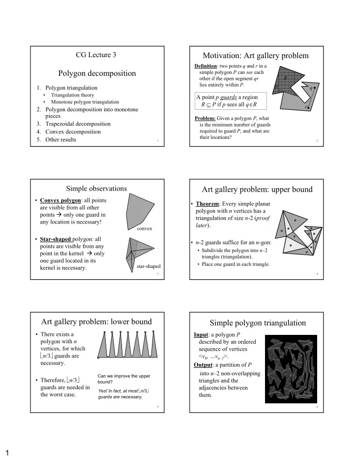
Motivation: Art gallery problem Motivation: Art gallery problem

Problem: Given a polygon P, what is the minimum number of guards required to guard P, and what are their locations? r q p R Definition: two points q and r in a simple polygon P can see each

• ther if the open segment qr

lies entirely within P.

A point p guards a region R ⊆ P if p sees all q∈R

3

Simple observations Simple observations

• Convex polygon: all points

are visible from all other points only one guard in any location is necessary!

• Star-shaped polygon: all

points are visible from any point in the kernel only

• ne guard located in its

kernel is necessary.

convex star-shaped

4

Art gallery problem: upper bound Art gallery problem: upper bound

• Theorem: Every simple planar

polygon with n vertices has a triangulation of size n-2 (proof later).

• n-2 guards suffice for an n-gon:
• Subdivide the polygon into n–2

triangles (triangulation).

• Place one guard in each triangle.

5

Art gallery problem: lower bound Art gallery problem: lower bound

• There exists a

polygon with n vertices, for which ⎣n/3⎦ guards are necessary.

• Therefore, ⎣n/3⎦

guards are needed in the worst case.

Can we improve the upper Can we improve the upper bound? bound? Yes! In fact, at most Yes! In fact, at most ⎣n/3⎦ guards are necessary. guards are necessary.

6

Simple polygon triangulation Simple polygon triangulation

Input: a polygon P described by an ordered sequence of vertices <v0, …vn–1>. Output: a partition of P into n–2 non-overlapping triangles and the adjacencies between them.

2

7

Simple polygon triangulation: observations Simple polygon triangulation: observations

• The triangulation is not unique. One of them

suffices.

• The triangulation is always possible.
• No new vertices are required.
• The triangulation adds new edges, called

diagonals, between existing vertices.

Not all diagonals are valid! Not all diagonals are valid!

8

Ideas? Ideas?

9

Triangulation theory Triangulation theory

• A vertex is convex if its interior angle < π,
• therwise it is concave.
• A diagonal is a new edge between two polygon

vertices that is entirely inside the polygon.

• Lemma 1: every polygon has a convex vertex.

Proof: the highest vertex (the one with the largest y coordinate) is convex.

• Lemma 2: Every polygon with n>3 vertices has

a diagonal.

10

Diagonals in polygons Diagonals in polygons

Proof: let v be a convex vertex and let a and b its adjacent vertices. Since P is a simple polygon and n>3, there is no edge between a and b. Consider the following two cases:

• 1. the new edge ab is a diagonal
• 2. Otherwise, there exists a vertex x

which is the closest to v with respect to a line L parallel to ab which is a diagonal. a a b b v v a a b b v v x x L L

Case 1 Case 1 Case 2 Case 2

11

Triangulation theory Triangulation theory

Theorem: Every simple polygon with n vertices has a triangulation with n–3 diagonals and n–2 triangles. Proof: By induction on n:

• Basis: A triangle (n=3) has a

triangulation (itself) with no diagonals and one triangle.

• Induction on n:

For an n-vertex polygon, construct a diagonal dividing the polygon into two polygons P1 and P2 with n1 and n2 vertices such that n1+n2–2 = n. Diagonals: (n1–3)+(n2 –3)+1 = (n1+n2–2)–3 = n–3 Triangles: (n1–2)+(n2–2) = (n1+n2–2)–2 = n–2

P P1

1

P P2

2

v v

12

Triangulation dual Triangulation dual

Definition: The triangulation dual T

• f a triangulation of a simple

polygon P is a graph whose nodes are triangles and whose edges are adjacencies between triangles sharing an edge. Property: the triangulation dual is a tree whose node degree is ≤ 3. Proof:

• Degree ≤ 3 by construction: no triangle has more than

three neighbors.

• No cycles: by contradiction. If it has a cycle, it is a

polygon with a hole (not a simple polygon).

• If fact,

If fact, T T is a binary tree with root degree one or two! is a binary tree with root degree one or two!

3

13

Simple triangulation algorithm (1) Simple triangulation algorithm (1)

Idea: Reduce the polygon by clipping a triangle at each iteration. The clipped triangle will be formed by three consecutive vertices (vi,vi+1,vi+2). The diagonal is (vi,vi+2). Test for validity: 1. The diagonal does not intersect other polygon edges. 2. The diagonal must be inside the polygon (test that diagonal is inside normal cone).

14

Simple triangulation algorithm Simple triangulation algorithm

proc triangulate(P) if |P| ≤ 3 output(P) and return; i 0; while diagonal(vi,vi+2) is not legal i++;

• utput(vi,vi+1,vi+2);

remove vi+1 from P; triangulate(P); Complexity: n times n diagonal tests that take each O(n) O(n3). Sources of inefficiencies:

• repeated diagonal tests
• diagonals are not sorted or ordered

Precompute diagonals in O(n2).

v v0 v v1

1

v v2

2

15

Triangulation algorithms Triangulation algorithms

• What is the lower bound?
• O(n2) by precomputing diagonals
• Improve to O(nlogn) by ordering them (see later).
• Is less than O(nlogn) possible?

17

O( O(n n log log n n) )-

• time triangulation algorithm

time triangulation algorithm

1) Partition the polygon into y-monotone pieces (“תוינו טונומ תוכיתח”). 2) Triangulate each y-monotone piece separately.

18

Monotone polygons: definition Monotone polygons: definition

• A simple polygon is called

monotone with respect to a line L if for any line L’ perpendicular to L the intersection of the polygon with L’ is connected.

• A polygon is called monotone if

there exists any such line ℓ.

• A polygon that is monotone with

respect to the x/y-axis is called x/y- monotone.

y-monotone but not x-monotone polygon Question: How can we check in O(n) time whether a polygon is y-monotone?

L L L L

19

Property of monotone polygons Property of monotone polygons

Definition: a vertex v is an interior cusp iff it is a concave vertex whose adjacent vertices are both at or above (at

• r below) line L.

Theorem: If a polygon P has no interior cusps with respect to a line L, then it is monotone with respect to L. Proof sketch: partition P into two chains connecting the top and bottom vertices. Assume one of them is not monotone with respect to L. Then P must contain an interior cusp above or below. v v v v L L

4

20

Triangulating a y Triangulating a y-

• monotone polygon

monotone polygon

• Sweep the polygon from top to bottom.
• Greedily triangulate anything possible above the

sweep line, and then forget about this region.

• When procesing a vertex v, the unhandled region

above it always has a simple structure: Two y-monotone (left and right) chains, each containing at least one edge. If a chain consists of two

• r more edges, it is reflex, and the other chain consists
• f a single edge whose bottom endpoint has not been

handled yet.

• Each diagonal is added in O(1) time.

21

Triangulating a Y Triangulating a Y-

• monotone polygon

monotone polygon

• Continue sweeping while one

chain contains only one edge, while the other edge is concave.

• When a “convex edge” appears

in the concave chain (or a second edge appears in the other

• ne), triangulate as much as

possible using a “fan”.

• Time complexity: O(k), where k

is the complexity of the polygon.

left chain left chain right chain right chain bottom bottom top top

22

Stack operations on chains Stack operations on chains

23

Monotone polygon triangulation Monotone polygon triangulation

24

Y Y-

• monotone polygons

monotone polygons

Polygon vertices classification:

• A start (resp., end) vertex is a

vertex whose interior angle is less than π and its two neighboring vertices both lie below (resp., above) it.

• A split (resp., merge) vertex is a

vertex whose interior angle is greater than π and its two neighboring vertices both lie below (resp., above) it.

• All other vertices are regular.

regular end start merge split

25

Vertex classification Vertex classification

5

26

Y Y-

• monotone polygons: properties

monotone polygons: properties

Theorem: A polygon without split and merge vertices is y-monotone. Proof: Since there are only start/end/regular vertices, the polygon must consist of two y-monotone chains. Alternatively, do a case analysis.

• To partition a polygon to monotone pieces,

eliminate split (merge) vertices by adding diagonals upward (downward) from the vertex. Naturally, the diagonals must not intersect!

regular end start merge split

27

Split and merge vertices Split and merge vertices

28

• Classify all vertices.
• Sweep the polygon from top to bottom.
• Maintain the edges intersected by the

sweep line L sorted by x coordinate).

• Maintain vertex events in an event queue

Q sorted by y coordinate.

• Eliminate split/merge vertices by

connecting them to other vertices.

• For each edge e, define helper(e) as the

lowest vertex (seen so far) above the sweep line visible to the right of the edge.

• helper(e) is initialized by the upper

endpoint of e.

Monotone partitioning Monotone partitioning

ej

helper(ej)

ek ei-1 ei vi

29

Monotone partitioning (cont.) Monotone partitioning (cont.)

• A split vertex may be connected

to the helper vertex of the edge immediately to its left.

• However, a merge vertex should

be connected to a vertex which has not been processed yet!

• Clever idea: Every merge vertex

is the helper of some edge, and will be handled when this edge “terminates”.

ej

helper(ej)

ek ej

helper(ej)

ek ei vi vi vm

30

Monotone partitioning algorithm Monotone partitioning algorithm

Input: A counterclockwise ordered list of vertices. The edge ei immediately follows the vertex vi. Construct Q on the vertices of P using y-coordinates. (when two or more vertices have the same y-coordinates, the vertex with the smaller x-coordinate has priority.)

• Initialize L to be empty.
• While Q is not empty:
• Pop vertex v;
• Handle v.

Note: No new events are generated during execution. No split/merge vertex remains unhandled.

31

Handling a start vertex vi:

• Add ei to L
• helper(ei)  vi

e1 e2 e3 e4 e5 e6 e7 e8 e9 v2 v3 v4 v5 v6 v7 v8 v9

Monotone partitioning Monotone partitioning

v1

6

32

Handling an end vertex vi:

• If helper(ei-1) is a merge

vertex, then connect vi to helper(ei-1)

• Remove ei-1 from L

e1 e2 e3 e4 e5 e6 e7 e8 e9 v2 v3 v4 v5 v6 v7 v8 v9

Monotone partitioning Monotone partitioning

v1

33

Handling a split vertex vi:

• Find in L the edge ej

directly to the left of vi

• Connect vi to helper(ej)
• helper(ej)  vi
• Insert ei into L
• helper(ei)  vi

e1 e2 e3 e4 e5 e6 e7 e8 e9 v2 v3 v4 v5 v6 v7 v8 v9

Monotone partitioning Monotone partitioning

v1

34

e1 e2 e3 e4 e5 e6 e7 e8 e9 v2 v3 v4 v5 v6 v7 v8

Monotone partitioning Monotone partitioning

v9

Handling a merge vertex vi:

• If helper(ei-1) is a merge

vertex, then connect vi to helper(ei-1)

• Remove ei-1 from L
• Find in L the edge ej

directly to the left of vi

• If helper(ej) is a merge vertex,

then connect vi to helper(ej)

• helper(ej)  vi

v1

35

v2 v7

Monotone partitioning Monotone partitioning

Handling a regular vertex vi:

• If the polygon’s interior lies to

the left of vi then:

• Find in L the edge ej directly to the

left of vi

• If helper(ej) is a merge vertex, then

connect vi to helper(ej)

• helper(ej)  vi
• Else:
• If helper(ei-1) is a merge vertex,

then connect vi to helper(ei-1)

• Remove ei-1 from L
• Insert ei into L
• helper(ei)  vi

e6 e7

36

Monotone polygon algorithm Monotone polygon algorithm

37

Event handling (1) Event handling (1)

7

38

Event handling (2) Event handling (2)

39

Example Example

40

Time complexity of polygon triangulation Time complexity of polygon triangulation

• Partitioning the polygon into monotone pieces:

O(n log n)

• Triangulating all the monotone pieces: O(n)
• Total:

O(n log n)

41

Trapezoidal decomposition Trapezoidal decomposition

• Decompose a polygon ito

trapezoids with two edges perpendicular to a give line.

• Trapezoids are trivially triangulated
• BUT – we need new intermediate

vertices.

• Useful for point search and other

tasks.

• Obtained directly from a sweep line

algorithm: at each vertex, compute the new supporting vertices left and

• right. Close trapezoids according to

neighborhood relations.

42

Convex partitioning Convex partitioning

Problem: partition a polygon P into a small (fewest) number of convex pieces. Possibilities:

• Use only vertices of P
• Use only vertices on edges of P
• Use new internal vertices (Steiner points)

Theorem: The smallest number of convex pieces λ that is needed to partition P is: ⌠r/2⌠ + 1 ≤ λ ≤ r + 1

where r is the number of concave vertices.

43

Hertl Hertl and and Melhorn Melhorn algorithm algorithm

Idea: triangulate polygon, then remove “non-essential”

• diagonals. A diagonal is non-

essential if its removal creates non-convexities. Note: only concave vertices have essential diagonals! Complexity: O(n log n) for triangulation. Is this strategy optimal? NO! Theorem: the number of pieces is never worse than four times the

• ptimal.

8

44

Other results Other results

• Optimal O(n) triangulation algorithm [Chazelle 1991]
• Finding the minimum number of guards for a simple

polygon is NP-hard [Aggarwal, 1984].

• 3D version: find a tetrahedrization of a simple

polyhedra.

• Not always possible without introducing new

vertices!

• The decision problem (are new vertices

necessary?) Is NP-complete.

• Algorithm runs in O(nr + r2 log r) time

[Chazelle and Palios, 1990].