= + N 1 N M measurements M 1 sparse signal Problem : Solve for - - PowerPoint PPT Presentation

Sparse processing / Compressed sensing

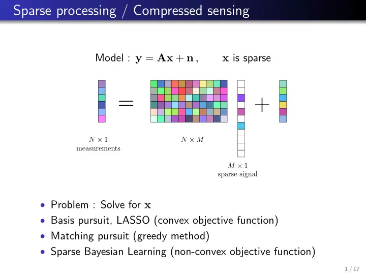
Model : y = Ax + n , x is sparse

=

N × 1 measurements N × M M × 1 sparse signal

+

• Problem : Solve for x
• Basis pursuit, LASSO (convex objective function)
• Matching pursuit (greedy method)
• Sparse Bayesian Learning (non-convex objective function)

1 / 17

The unconstrained -LASSO- formulation

Constrained formulation of the `1-norm minimization problem:

b x`1() = arg min

x2CN kxk1 subject to ky − Axk2 ≤

Unconstrained formulation in the form of least squares optimization with an `1-norm regularizer:

b xLASSO(µ) = arg min

x2CN

ky − Axk2

2 + µkxk1

For every exists a µ so that the two formulations are equivalent

Regularization parameter :

µ

2 / 17

Bayesian interpretation of unconstrained LASSO

Bayes rule : Maximum a posteriori (MAP) estimate :

3 / 17

Bayesian interpretation of unconstrained LASSO

Gaussian likelihood : Laplace Prior : MAP estimate :

4 / 17

Bayesian interpretation of unconstrained LASSO

MAP estimate :

5 / 17

Prior and Posterior densities (Ex. Murphy)

6 / 17

Sparse Bayesian Learning (SBL)

Model : y = Ax + n Prior : x ∼ N(x; 0, Γ) Γ = diag(γ1, . . . , γM) Likelihood : p(y|x) = N(y; Ax, σ2IN)

=

N × 1 measurements N × M M × 1 sparse signal

+

Evidence : SBL solution :

M.E.Tipping, ”Sparse Bayesian learning and the relevance vector machine,” Journal of Machine Learning Research, June 2001. 7 / 17

SBL overview

• SBL solution : ˆ

Γ = arg min

Γ

• log |Σy| + yHΣ−1

y y

• SBL objective function is non-convex
• Optimization solution is non-unique
• Fixed point update using derivatives, works in practice
• Γ = diag(γ1, . . . , γM)

Update rule : γnew

m

= γold

m

||yHΣ−1

y am||2 2

aH

mΣ−1 y am

Σy = σ2IN + AΓAH

• Multi snapshot extension : same Γ across snapshots

8 / 17

SBL overview

• Posterior : xpost = ΓAHΣ−1

y y

• At convergence, γm → 0 for most γm
• Γ controls sparsity, E(|xm|2) = γm
• Different ways to show that SBL gives sparse output
• Automatic determination of sparsity
• Also provides noise estimate σ2

9 / 17

• 90
• 70
• 50
• 30
• 10

10 30 50 70 90 Angle 3 (° ) 50 100 150 . (3)

iteration #0

Applications to acoustics - Beamforming

• Beamforming
• Direction of arrivals (DOAs)

10 / 17

SBL - Beamforming example

• N = 20 sensors, uniform linear array
• Discretize angle space: {−90 : 1 : 90}, M = 181
• Dictionary A : columns consist of steering vectors
• K = 3 sources, DOAs, [−20, −15, 75]◦, [12, 22, 20] dB
• M ≫ N > K

10 20

P (dB)

CBF

• 90
• 70
• 50
• 30
• 10

10 30 50 70 90 Angle 3 (° ) 10 20 . (dB)

SBL

11 / 17

SBL - Acoustic hydrophone data processing (from Kai)

CBF SBL Eigenrays Ship of Opportunity

12 / 17

Problem with Degrees of Freedom

• As the number of snapshots (=observations) increases, so does the

number of unknown complex source amplitudes

• PROBLEM: LASSO for multiple snapshots estimates the realizations of

the random complex source amplitudes.

• However, we would be satisfied if we just estimated their power

γm = E{ |xml|2 }

• Note that γm does not depend on snapshot index l.

Thus SBL is much faster than LASSO for more snapshots.

13 / 17

Example CPU Time

1 10 100 1000 Snapshots 0.1 1 10 200 CPU time (s)

b)

SBL SBL1 LASSO

1 10 100 1000 Snapshots 0.2 0.4 0.6 0.8 1 DOA RMSE [°]

c)

SBL SBL1 LASSO

LASSO use CVX, CPU∝L2 SBL nearly independent on snapshots

14 / 17

Matching Pursuit

Model : y = Ax + n , x is sparse

=

N × 1 measurements N × M M × 1 sparse signal

+

• Greedy search method
• Select column that is most aligned with the current residual

15 / 17

16 / 17

If the magnitudes of the non-zero elements in x0 are highly

scaled, then the canonical sparse recovery problem should be easier.

The (approximate) Jeffreys distribution produces

sufficiently scaled coefficients such that best solution can always be easily computed.

Amplitude Distribution

x0 x0

For strongly scaled coefficients, Matching Pursuit (or Orthogonal MP) works better. It picks one coefficient at a time.

17 / 17