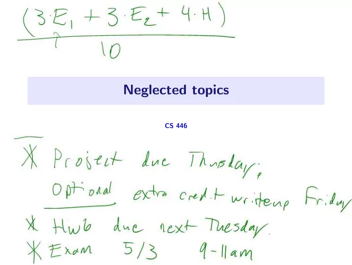
Neglected topics CS 446 Adversarial examples and deep networks 1 / - - PowerPoint PPT Presentation

Neglected topics

CS 446

Adversarial examples and deep networks

1 / 23

“Adversarial examples”?

◮ Standard ML setup:

◮ We have training data; try to do well on withheld testing data.

◮ Adversarial/robust ML setup:

◮ We have training data; try to do well on small perturbations of training and testing data.

2 / 23

“Adversarial examples”?

◮ Standard ML setup:

◮ We have training data; try to do well on withheld testing data.

◮ Adversarial/robust ML setup:

◮ We have training data; try to do well on small perturbations of training and testing data.

◮ This is an old problem (see for instance “robust statistics”). ◮ For deep networks, it has been rekindled for the following reasons:

◮ Deep networks have absurdly good performance on training and test error, comparable to humans. ◮ Unlike humans, deep networks completely choke on small perturbations.

◮ Some background reading:

◮ Original paper: “Intriguing properties of neural networks”; Christian Szegedy, Wojciech Zaremba, Ilya Sutskever, Joan Bruna, Dumitru Erhan, Ian Goodfellow, Rob Fergus; https://arxiv.org/abs/1312.6199. ◮ Nice theory overview: video lecture by Sebastien Bubeck https://www.youtube.com/watch?v=9flSRJdnWek.

2 / 23

Adversarial examples in computer vision

(“Explaining and harnessing adversarial examples”; Ian J. Goodfellow, Jonathon Shlens, Christian Szegedy.) ◮ Can make a small change humans can’t see, and fool an otherwise impressive deep network. ◮ There are versions that are “physical”, e.g., you wear special 3-d printed glasses and fool a deep-network-based security system.

◮ This is one reason self-driving cars are scary, but there are others. (The death caused by an Uber self-driving car was not due to a deep network.)

3 / 23

Formal statement of problem

◮ Training loss: ℓ(f(x), y). ◮ Adversarial training loss (ℓ∞ is popular): max

p∞≤δ ℓ(f(x + p), y)

◮ By making δ small and solving for p, we can find an imperceptible adversarial perturbation. ◮ There are many variations; e.g., forcing us to switch the label to a specific y′ (“targeted attacks”). ◮ Finding an adversarial example means solving this maximization

• problem. There’s a lot of research into this, it seems to boil down to

gradient descent (ascent) variants.

4 / 23

Defenses

◮ Finding ways to make networks robust is a big research area (“defenses against these attacks”). ◮ Natural approach: do ERM on the adversarial loss: min

f∈F

1 n

n

• i=1

max

pi∞≤δ ℓ

• f(xi + pi), yi
• .

(From “Towards deep learning models resistant to adversarial attacks” by Aleksander Madry, Aleksandar Makelov, Ludwig Schmidt, Dimitris Tsipras, Adrian Vladu.)

5 / 23

Other comments

◮ Big research area (both attacks and defenses). ◮ Lots of hype (this is good and bad). ◮ Isn’t just an issue with deep networks; but it’s interesting to know what parts of the question are due to them. ◮ Might motivate changes in training algorithms.

6 / 23

Time series

7 / 23

Time series

◮ Rather than having IID ((x1, y1), . . . , (xn, yn)), we either have:

◮ ((x1, y1), . . . , (xn, yn)) where (xi+1, yi+1) uses (xi, yi) (“Markov assumption”), or even more history. ◮ Multiple “traces”: we collect m time series, with lengths (t1, . . . , tm):

• (x(j)

i , y(j) i )

tj

i=1

m

j=1

.

◮ This is an extremely classical topic with many approaches inside and

• utside ML.

◮ E.g., the signal processing community; look up “auto-regressive model” for a basic approach (linear). ◮ We skipped/rushed the Hidden Markov Model (HMM) slides, which give a graphical model formulation and approach. ◮ Recurrent neural networks (RNNs) are another approach. ◮ ML Theory community is behind on this topic (e.g., a “generalization bound” that doesn’t grow quickly with length tj). I’m not sure why.

8 / 23

Recurrent neural networks (RNNs)

◮ The model is based on a deep network f.

◮ At time i we get both an input xi, and a state vector si. ◮ We compute (yi, si+1) = f(xi, si), where yi is our output, and si+1 is the state vector consumed in the next round.

◮ Popular choice of f: “Long short-term memory (LSTM)”. ◮ Example: consume English words, output Japanese words.

◮ There are all sorts of issues with this; for instance, words should not be in 1-to-1 mapping! ◮ Most language stuff these days uses a “BiLSTM”, but I’ve also heard

• f people using multi-layer 1-d conv equivalently well.

9 / 23

Reinforcement learning (RL)

10 / 23

RL setup

◮ We are again in the time series setup (x1, . . .), but:

◮ Our choices affect future x ! ◮ There are no clear losses/rewards; people talk about “rewards”, “feedback”, and “reinforcement”.

◮ There are many variants of the problem with many approaches.

◮ Some problems can be solved with a deterministic approach; dynamic programming was proposed by Bellman for reinforcement learning problems, and “Bellman equation” still fundamental in RL. ◮ For some other classical ideas, look up “MDP” and “POMDP”.

11 / 23

Chess example

◮ Very few moves actually result in feedback (checkmate or draw).

◮ We can work backwards from such moves to assign scores. ◮ This is computationally prohibitive, but some people have tried (look up “chess tablebase”). ◮ This is too conservative against weak opponents.

◮ Despite this, we can “guess” feedback, either deterministically, or “statistically” (as in course project).

◮ We can also “improve” such an estimate by playing against ourself and averaging the outcomes (“Monte-Carlo Tree Search (MCTS)”). ◮ If instead we form upper and lower bounds on the outcome and descend the game tree to refine them, it is called “alpha-beta search”.

12 / 23

Chess example (continued)

Here’s an alternating approach to chess RL (used by “alphago zero”):

• 1. Fix the evaluation/scoring function f, and play games against self

using MCTS (which improves the scoring function).

• 2. Go over the games, and fit f to the move choices with standard

supervised learning (course project suggests only this step). To train, alternate steps 1 and 2. To “test”/play, do step 1. (“AlphaGo Zero cheatsheet”, not by me.)

13 / 23

(“AlphaGo Zero cheatsheet”, not by me; larger version.)

14 / 23

Resources

◮ This is a huge field with not just many approaches, but many styles

• f approaches from many different fields (not just CS or ML even).

◮ The Berkeley “Deep RL” course presents some cutting-edge material and also links to many other resources: http://rail.eecs.berkeley.edu/deeprlcourse/ . ◮ Theoretical simplification of the problem: bandit algorithms.

15 / 23

Natural language processing (NLP)

16 / 23

Natural language processing (NLP)

◮ This is a big application area concerned with human text. ◮ Most basic approach: rewrite task as supervised learning from Rd to Rk.

◮ Input encoding #1: “bag of words” (document becomes normalized vector of per-word counts); effective for easy problems. ◮ Input encoding #2: Word2Vec (a standard deep network that has become a very standard way to encode words).

◮ Cutting-edge approaches now use word-level and even character-level deep networks (or recurrent networks), with complicated outputs (tasks like a sequence of question-answer pairs). ◮ For more info, see this recent stanford NLP class: https://web.stanford.edu/class/cs224n/.

17 / 23

Dealing with data

18 / 23

Dealing with data

◮ Data cleaning/normalizing: a huge issue which could break everything we’ve discussed if it is ignored.

◮ Another issue is missing data/entries. People used to use EM for this, but I’m not sure what’s current practice?

◮ Data augmentation.

◮ For CIFAR, it’s standard to thrown in random crops and flips.

◮ pytorch provides tools for data cleaning and augmentation (look up torchvision.transforms).

19 / 23

Why are deep networks dominating?

20 / 23

Why are deep networks dominating?

◮ I don’t think anyone really knows. Certainly, no one has good predictive power (why didn’t we use ReLU, batch norm, and convnets when they were discovered in the 1970s?).

21 / 23

Why are deep networks dominating?

◮ I don’t think anyone really knows. Certainly, no one has good predictive power (why didn’t we use ReLU, batch norm, and convnets when they were discovered in the 1970s?). ◮ A few reasons:

◮ They seems to succinctly approximate many natural phenomena, perhaps due to some underlying compositional/hierarchical structure. ◮ They seem to work well with recent hardware coincidences (“GPU” was not designed for deep learning). ◮ They seem to work well with lots of data (at least, as they are trained now), and we now have lots of data. ◮ Gradient descent + deep networks = magic. ◮ The software infrastructure is amazing; “hacking” deep networks is somehow fun and accessible to basically every programmer. ◮ The momentum with the “social coding” ecosystem.

21 / 23

Other big neglected topics

22 / 23

Other big neglected topics

◮ Interpretability (crucial for many applications, including medicine and law). ◮ Applications-specific issues (e.g., in audio, robotics, . . . ).

23 / 23