[PPT] - Network Flow II 2 Every edge e has a capacity c(e) 0. Flow: 1 PowerPoint Presentation

SLIDE 1

Network Flow II

Inge Li Gørtz

KT 7.3, 7.5, 7.6

1

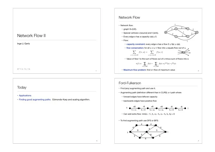
Network Flow

Network flow:
graph G=(V,E).
Special vertices s (source) and t (sink).
Every edge e has a capacity c(e) ≥ 0.
Flow:
capacity constraint: every edge e has a flow 0 ≤ f(e) ≤ c(e).
flow conservation: for all u ≠ s, t: flow into u equals flow out of u.
Value of flow f is the sum of flows out of s minus sum of flows into s:
Maximum flow problem: find s-t flow of maximum value

1 2 2 2 2 1 2 2 1 s t

X

v:(v,u)∈E

f(v, u) = X

v:(u,v)∈E

f(u, v)

u

v( f ) = ∑

v:(s,v)∈E

f(e) − ∑

v:(v,s)∈E

f(e) = f out(s) − f in(s)

2

Today

Applications
Finding good augmenting paths. Edmonds-Karp and scaling algorithm.

3

Find (any) augmenting path and use it.
Augmenting path (definition different than in CLRS): s-t path where
forward edges have leftover capacity
backwards edges have positive flow
Can add extra flow: min(c1 - f1, f2, c3 - f3, c4 - f4, f5, f6) = δ
To find augmenting path use DFS or BFS:

Ford-Fulkerson

s t

f1 < c1 f2 > 0 f3 < c3 f4 < c4 f5 > 0 f6 > 0 +δ +δ +δ

δ
δ
δ

s

4 4 4 4 9 4 3 8 2 5 6 6

t

4

SLIDE 2

Integral capacities:
Each augmenting path increases flow with at least 1.
At most v(f) iterations
Find augmenting path via DFS/BFS: O(m)
Total running time: O(v(f) m)
Lemma. If all the capacities are integers, then there is a maximum flow where the

flow on every edge is an integer.

Bad example for Ford-Fulkerson:

Ford-Fulkerson

s

1.000.000 1.000.000 1.000.000 1.000.000 1 1/ 1/ 1/ 1/ 1/ 0/ 1/ 2/ 2/ 2/ 2/ 0/

5

Find shortest augmenting path and use it.
Augmenting path (definition different than in CLRS): s-t path where
forward edges have leftover capacity
backwards edges have positive flow
Can add extra flow: min(c1 - f1, f2, c3 - f3, c4 - f4, f5, f6) = δ
To find augmenting path use BFS:

Edmonds-Karp

s t

f1 < c1 f2 > 0 f3 < c3 f4 < c4 f5 > 0 f6 > 0 +δ +δ +δ

δ
δ
δ

s

4 4 4 4 9 4 3 8 2 5 6 6

t

3/ 3/

6

Find shortest augmenting path and use it.
Augmenting path (definition different than in CLRS): s-t path where
forward edges have leftover capacity
backwards edges have positive flow
Can add extra flow: min(c1 - f1, f2, c3 - f3, c4 - f4, f5, f6) = δ
To find augmenting path use BFS:

Edmonds-Karp

s t

f1 < c1 f2 > 0 f3 < c3 f4 < c4 f5 > 0 f6 > 0 +δ +δ +δ

δ
δ
δ

s

4 4 4 4 3/9 4 3/3 8 2 5 6 6

7

Find shortest augmenting path and use it.
Augmenting path (definition different than in CLRS): s-t path where
forward edges have leftover capacity
backwards edges have positive flow
Can add extra flow: min(c1 - f1, f2, c3 - f3, c4 - f4, f5, f6) = δ
To find augmenting path use BFS:

Edmonds-Karp

s t

f1 < c1 f2 > 0 f3 < c3 f4 < c4 f5 > 0 f6 > 0 +δ +δ +δ

δ
δ
δ

s

4 4 4 4/4 7/9 4/4 3/3 8 2 5 6 6

8

SLIDE 3

Find shortest augmenting path and use it.
Augmenting path (definition different than in CLRS): s-t path where
forward edges have leftover capacity
backwards edges have positive flow
Can add extra flow: min(c1 - f1, f2, c3 - f3, c4 - f4, f5, f6) = δ
To find augmenting path use BFS:

Edmonds-Karp

s t

f1 < c1 f2 > 0 f3 < c3 f4 < c4 f5 > 0 f6 > 0 +δ +δ +δ

δ
δ
δ

s

4 4 4 4/4 9/9 4/4 3/3 2/8 2 2/5 2/6 6

9

Find shortest augmenting path and use it.
Augmenting path (definition different than in CLRS): s-t path where
forward edges have leftover capacity
backwards edges have positive flow
Can add extra flow: min(c1 - f1, f2, c3 - f3, c4 - f4, f5, f6) = δ
To find augmenting path use BFS:

Edmonds-Karp

s t

f1 < c1 f2 > 0 f3 < c3 f4 < c4 f5 > 0 f6 > 0 +δ +δ +δ

δ
δ
δ

s

3/4 3/4 3/4 4/4 9/9 1/4 3/3 5/8 2 5/5 5/6 6

10

When there are no more augmenting s-t paths:
Find all augmenting paths from s.
The nodes S that can be reached by these augmenting paths form the left side of a

minimum cut.

edges out of S have ce = fe.
edges into S have fe = 0.
Capacity of the cut equals the flow.

Find a minimum cut

s

3/4 3/4 3/4 4/4 9/9 1/4 3/3 5/8 2 5/5 5/6 6

11

Scaling parameter Δ
Only consider edges with capacity at least Δ in residual graph Gf(Δ).
Example: Δ = 4

Scaling algorithm

Gf(4) Gf

s

1 1 1 4 4 1 3 4 2 2 2 6

t

3 3 3 3 5 4 4 4

s

1 1 1 4 4 1 3 4 2 2 2 6

t

3 3 3 3 5 4 4 4

12

SLIDE 4

Scaling algorithm

Scaling parameter Δ
Only consider edges with capacity at least Δ in residual graph Gf(Δ).
Start with Δ = “highest power of 2 ≤ largest capacity out of s”

6 9 13 10 1 8 4 3 2 5 Δ = 8

s t

13

Scaling algorithm

Scaling parameter Δ
Only consider edges with capacity at least Δ in residual graph Gf(Δ).
Start with Δ = “highest power of 2 ≤ largest capacity out of s”

6 9 13 10 1 8 4 3 2 5 Δ = 8

s t

14

Scaling algorithm

Scaling parameter Δ
Only consider edges with capacity at least Δ in residual graph Gf(Δ).
Start with Δ = “highest power of 2 ≤ largest capacity out of s”

6 9 13 10 1 8 4 3 2 5 Δ = 8 9/ 9/ 9/

s t

15

Scaling algorithm

Scaling parameter Δ
Only consider edges with capacity at least Δ in residual graph Gf(Δ).
Start with Δ = “highest power of 2 ≤ largest capacity out of s”

6 9 4 1 1 8 4 3 2 5 Δ = 8 9 9

s t

16

SLIDE 5

Scaling algorithm

Scaling parameter Δ
Only consider edges with capacity at least Δ in residual graph Gf(Δ).
Start with Δ = “highest power of 2 ≤ largest capacity out of s”
When no more augmenting paths in Gf(Δ): Δ = Δ/2 (new phase).

6 9 4 1 1 8 4 3 2 5 Δ = 8 9 9

s t

17

Scaling algorithm

Scaling parameter Δ
Only consider edges with capacity at least Δ in residual graph Gf(Δ).
Start with Δ = “highest power of 2 ≤ largest capacity out of s”
When no more augmenting paths in Gf(Δ): Δ = Δ/2 (new phase).

6 9 4 1 1 8 4 3 2 5 Δ = 4 9 9

s t

18

Scaling algorithm

Scaling parameter Δ
Only consider edges with capacity at least Δ in residual graph Gf(Δ).
Start with Δ = “highest power of 2 ≤ largest capacity out of s”
When no more augmenting paths in Gf(Δ): Δ = Δ/2 (new phase).

6 9 4 1 1 8 4 3 2 5 Δ = 4 9 9

s t

4/ 4/ 4/ 4/ 4/

19

Scaling algorithm

Scaling parameter Δ
Only consider edges with capacity at least Δ in residual graph Gf(Δ).
Start with Δ = “highest power of 2 ≤ largest capacity out of s”
When no more augmenting paths in Gf(Δ): Δ = Δ/2 (new phase).

2 9 4 5 1 4 4 3 2 1 Δ = 4 9 5

s t

4 4 4

20

SLIDE 6

Scaling algorithm

Scaling parameter Δ
Only consider edges with capacity at least Δ in residual graph Gf(Δ).
Start with Δ = “highest power of 2 ≤ largest capacity out of s”
When no more augmenting paths in Gf(Δ): Δ = Δ/2 (new phase).

2 9 4 5 1 4 4 3 2 1 Δ = 4 9 5

s t

4 4 4

21

Scaling algorithm

Scaling parameter Δ
Only consider edges with capacity at least Δ in residual graph Gf(Δ).
Start with Δ = “highest power of 2 ≤ largest capacity out of s”
When no more augmenting paths in Gf(Δ): Δ = Δ/2 (new phase).

2 9 4 5 1 4 4 3 2 1 Δ = 2 9 5

s t

4 4 4

22

Scaling algorithm

Scaling parameter Δ
Only consider edges with capacity at least Δ in residual graph Gf(Δ).
Start with Δ = “highest power of 2 ≤ largest capacity out of s”
When no more augmenting paths in Gf(Δ): Δ = Δ/2 (new phase).

2 9 4 5 1 4 4 3 2 1 Δ = 2 9 5

s t

4 4 4 2/ 2/ 2/

23

Scaling algorithm

Scaling parameter Δ
Only consider edges with capacity at least Δ in residual graph Gf(Δ).
Start with Δ = “highest power of 2 ≤ largest capacity out of s”
When no more augmenting paths in Gf(Δ): Δ = Δ/2 (new phase).

9 4 7 1 4 4 1 2 1 Δ = 2 9 3

s t

6 4 4 2

24

SLIDE 7

Scaling algorithm

Scaling parameter Δ
Only consider edges with capacity at least Δ in residual graph Gf(Δ).
Start with Δ = “highest power of 2 ≤ largest capacity out of s”
When no more augmenting paths in Gf(Δ): Δ = Δ/2 (new phase).

9 4 7 1 4 4 1 2 1 Δ = 2 9 3

s t

6 4 4 2

25

Scaling algorithm

Scaling parameter Δ
Only consider edges with capacity at least Δ in residual graph Gf(Δ).
Start with Δ = “highest power of 2 ≤ largest capacity out of s”
When no more augmenting paths in Gf(Δ): Δ = Δ/2 (new phase).

9 4 7 1 4 4 1 2 1 Δ = 1 9 3

s t

6 4 4 2

26

Scaling algorithm

Scaling parameter Δ
Only consider edges with capacity at least Δ in residual graph Gf(Δ).
Start with Δ = “highest power of 2 ≤ largest capacity out of s”
When no more augmenting paths in Gf(Δ): Δ = Δ/2 (new phase).

9 4 7 1 4 4 1 2 1 Δ = 1 9 3

s t

6 4 4 2 1/ 1/

27

Scaling algorithm

Scaling parameter Δ
Only consider edges with capacity at least Δ in residual graph Gf(Δ).
Start with Δ = “highest power of 2 ≤ largest capacity out of s”
When no more augmenting paths in Gf(Δ): Δ = Δ/2 (new phase).

9 3 7 1 4 4 2 1 Δ = 1 10 3

s t

6 4 4 3

28

SLIDE 8

Scaling algorithm

Scaling parameter Δ
Only consider edges with capacity at least Δ in residual graph Gf(Δ).
Start with Δ = “highest power of 2 ≤ largest capacity out of s”
When no more augmenting paths in Gf(Δ): Δ = Δ/2 (new phase).

9 3 7 1 4 4 2 1 Δ = 1 10 3

s t

6 4 4 3 1/ 1/ 1/ 1/

29

Scaling algorithm

Scaling parameter Δ
Only consider edges with capacity at least Δ in residual graph Gf(Δ).
Start with Δ = “highest power of 2 ≤ largest capacity out of s”
When no more augmenting paths in Gf(Δ): Δ = Δ/2 (new phase).
Stop when no more augmenting paths in Gf(1).

9 3 7 1 5 4 1 1 Δ = 1 10 3

s t

6 3 4 3

30

Scaling algorithm

s

1.000.000 1.000.000 1.000.000 1.000.000 1

31

Scaling algorithm

s

1.000.000 1.000.000 1.000.000 1.000.000 1

s

1.000.000 1.000.000 1.000.000 1.000.000 1 1.000.000/ 1.000.000/ 1.000.000/ 1.000.000/

32

SLIDE 9

Scaling algorithm

s

1.000.000 1.000.000 1.000.000 1.000.000 1

s

1.000.000 1.000.000 1.000.000 1.000.000 1 1.000.000/ 1.000.000/ 1.000.000/ 1.000.000/ 1.000.000/ 1.000.000/

33

Scaling algorithm

s

1.000.000 1.000.000 1.000.000 1.000.000 1

s

1.000.000 1.000.000 1.000.000 1.000.000 1 1.000.000/ 1.000.000/ 1.000.000/ 1.000.000/

34

Scaling algorithm

s

1.000.000 1.000.000 1.000.000 1.000.000 1

s

1.000.000 1.000.000 1.000.000 1.000.000 1 1.000.000/ 1.000.000/ 1.000.000/ 1.000.000/

35

Exercise

s t A B C D 10 9 11 9 5 5 10 3 3 3 3

SLIDE 10

Running time: O(m2 log C), where C is the largest capacity out of s.
Lemma 1. Number of scaling phases: 1 +⎡lg C⎤
Lemma 2. Let f the flow when Δ-scaling phase ends, and let f*be the maximum flow.

Then v(f*) ≤ v(f) + mΔ.

Lemma 3. The number of augmentations in a scaling phase is at most 2m.
First phase: can use each edge out of s in at most one augmenting path.
f flow at the end of previous phase.
Used Δ’ = 2Δ in last round.
Lemma 2: v(f*) ≤ v(f) + mΔ’ = v(f) + 2mΔ.
“Leftover flow” to be found ≤ 2mΔ.
Each agumentation in a Δ-scaling phase augments flow with at least Δ.

Scaling algorithm

37

Lemma 2. Let f the flow when Δ-scaling phase ends, and let f*be the maximum flow.

Then v(f*) ≤ v(f) + mΔ.

By the end of the phase there is a cut c(S,T) ≤ v(f) + mΔ.

Scaling algorithm

s t S T

c(e)-f(e) < Δ f(e) < Δ e1 e3 e7 e5 e2

c(S, T) = c(e1) + c(e3) + c(e7) v( f ) = f(e1) + f(e3) + f(e7) − f(e2) − f(e5) c(S, T) − v( f ) = c(e1) + c(e3) + c(e7) − f(e1) − f(e3) − f(e7) + f(e2) + f(e5) = c(e1) − f(e1) + c(e3) − f(e3) + c(e7) − f(e7) + f(e2) + f(e5) < Δ + Δ + Δ + Δ + Δ = 5Δ

38

Edmonds-Karp: O(m2n)
Scaling: O(m2 log C)
Ford-Fulkerson O(m v(f)).
Preflow-push O(n3)
Other algorithms: O(mn log n) or O(min(n2/3, m1/2)m log n log U).

Maximum flow algorithms

39

Bipartite graph: Can color vertices red and blue such that all edges have a red and a

blue endpoint.

Matching: Subset of edges M ⊆ E such that no edges in M share an endpoint.
Maximum matching: matching of maximum cardinality.
Applications:
planes to routes
jobs to workers/machines

Maximum Bipartite Matching

Matching Maximum matching

matched

40

SLIDE 11

1 1 1 1 1 1 1

Bipartite graph: Can color vertices red and blue such that all edges have a red and a

blue endpoint.

Matching: Subset of edges M ⊆ E such that no edges in M share an endpoint.
Maximum matching: matching of maximum cardinality.
Solve via flow:

Maximum Bipartite Matching

s t

1

41

1 1 1 1 1 1 1

Bipartite graph: Can color vertices red and blue such that all edges have a red and a

blue endpoint.

Matching: Subset of edges M ⊆ E such that no edges in M share an endpoint.
Maximum matching: matching of maximum cardinality.
Solve via flow:
Matching M => flow of value |M|

Maximum Bipartite Matching

s t

1

42

1 1 1 1 1 1 1

Bipartite graph: Can color vertices red and blue such that all edges have a red and a

blue endpoint.

Matching: Subset of edges M ⊆ E such that no edges in M share an endpoint.
Maximum matching: matching of maximum cardinality.
Solve via flow:
Matching M => flow of value |M|

Maximum Bipartite Matching

s t

1

43

Bipartite graph: Can color vertices red and blue such that all edges have a red and a

blue endpoint.

Matching: Subset of edges M ⊆ E such that no edges in M share an endpoint.
Maximum matching: matching of maximum cardinality.
Solve via flow:
Matching M => flow of value |M|

1 1 1 1 1 1 1

Maximum Bipartite Matching

s t

1

44

SLIDE 12

Bipartite graph: Can color vertices red and blue such that all edges have a red and a

blue endpoint.

Matching: Subset of edges M ⊆ E such that no edges in M share an endpoint.
Maximum matching: matching of maximum cardinality.
Solve via flow:
Matching M => flow of value |M|
Flow of value v(f) => matching of size v(f)

1 1 1 1 1 1 1

Maximum Bipartite Matching

s t

1

45

Bipartite graph: Can color vertices red and blue such that all edges have a red and a

blue endpoint.

Matching: Subset of edges M ⊆ E such that no edges in M share an endpoint.
Maximum matching: matching of maximum cardinality.
Solve via flow:
Can generalize to general matchings

2 2 2 1 1 1 1

Maximum Bipartite Matching

s t

1

46

X doctors, Y holidays, each doctor should work at at most 1 holiday, each doctor is

available at some of the holidays.

Same problem, but each doctor should work at most c holidays?

Scheduling of doctors

Doctors Holidays

47

X doctors, Y holidays, each doctor should work at at most c holidays, each doctor is

available at some of the holidays.

Same problem, but each doctor should work at most one day in each vacation

period?

Scheduling of doctors

s t

1 1 c c c

48

SLIDE 13

X doctors, Y holidays, each doctor should work at at most c holidays, each doctor is

available at some of the holidays.

Same problem, but each doctor should work at most one day in each vacation

period?

Scheduling of doctors

s t

1 1 c c c

49

X doctors, Y holidays, each doctor should work at at most c holidays, each doctor is

available at some of the holidays.

Same problem, but each doctor should work at most one day in each vacation

period?

Scheduling of doctors

s t

1 1 c c c

50

Problem: Find maximum number of edge-disjoint paths from s to t.
Two paths are edge-disjoint if they have no edge in common.

Edge Disjoint paths

s t

51

Edge-disjoint path problem. Find the maximum number of edge-disjoint paths from

s to t.

Two paths are edge-disjoint if they have no edge in common.

Edge Disjoint paths

s t

52

SLIDE 14

Reduction to max flow: assign capacity 1 to each edge.
Thm. Max number of edge-disjoint s-t paths is equal to the value of a maximum

flow.

Suppose there are k edge-disjoint paths: then there is a flow of k (let all edges on

the paths have flow 1).

Other way (graph theory course).
Ford-Fulkerson: v(f) ≤ n (no multiple edges and therefore at most n edges out of s)

=> running time O(nm).

Edge Disjoint Paths

s t

1 1 1 1 1 1 1 1 1 1 1 1 1

53

Network connectivity. Find minimum number of edges whose removal disconnects t

from s (destroys all s-t paths).

Network Connectivity

s t

1 1 1 1 1 1 1 1 1 1 1 1 1

54

Network connectivity. Find minimum number of edges whose removal disconnects t

from s (destroys all s-t paths).

Set all capacities to 1 and find minimum cut.
Thm. (Menger) The maximum number of edge-disjoint s-t paths is equal to the

minimum number of edges whose removal disconnects t from s.

Network Connectivity

s t

1 1 1 1 1 1 1 1 1 1 1 1 1

55

Question: Can Boston finish in first place (or in tie of first place)?
No: Boston must win both its remaining 2 and NY must loose. But then Baltimore

and Toronto both beat NY so winner of Baltimore-Toronto will get 93 points.

Other argument: Boston can finish with at most 92. Cumulatively the other three

teams have 274 wins currently and their 3 games against each other will give another 3 points => 277. 277/3 = 92,33333 => one of them must win > 92.

Baseball elimination

56

Team Wins Games left Against NY Bal Tor Bos New York 92 2

1

1 Baltimore 91 3 1

1

1 Toronto 91 3 1 1

1

Boston 90 2 1 1

SLIDE 15

Baseball elimination

57

Team Wins Games left Against NY Bal Tor Bos New York 90 11

1

6 4 Baltimore 88 6 1

1

4 Toronto 87 11 6 1

4

Boston 79 12 4 4 4

Question: Can Boston finish in first place (or in tie of first place)?

s t

NY-Bal NY-Tor Tor-Bal NY Bal Tor 1 6 1

∞

1 = 91-90

Boston can get at most 79 + 12 = 91 points

3 4

Boston is eliminated ⇔ max s-t flow < 8.
Capacities on nodes.

Node capacities

⬇

c

v e d c b a

c

vin vout e d c b a

58