Notation ^ y = b 0 + b 1 x 1 + b 2 x 2 + b 3 x 3 +. . .+ b k x k 0 - - PDF document

notation
SMART_READER_LITE
LIVE PREVIEW

Notation ^ y = b 0 + b 1 x 1 + b 2 x 2 + b 3 x 3 +. . .+ b k x k 0 - - PDF document

Multiple Regression Multiple Regression Definition Definition Multiple Regression Equation Multiple Regression Equation A linear relationship between a dependent A linear relationship between a dependent variable y and two or more independent


slide-1
SLIDE 1

Multiple Regression

Definition

Multiple Regression Equation

A linear relationship between a dependent variable y and two or more independent variables (x1, x2, x3 . . . , xk) Model: y = ßo+ ß1x1+ ß2x2+ . . . ßkxk+e

Multiple Regression

Definition

Multiple Regression Equation

A linear relationship between a dependent variable y and two or more independent variables (x1, x2, x3 . . . , xk)

y = b0 + b1x1 + b2x2 + . . . + bkxk

^ y = b0 + b1 x1+ b2 x2+ b3 x3 +. . .+ bk xk

(General form of the estimated multiple regression equation)

n = sample size k = number of independent variables y = predicted value of the

dependent variable y

x1, x2, x3 . . . , xk are the independent

variables ^ ^

ß0 = the y-intercept, or the value of y when all

  • f the predictor variables are 0

b0 = estimate of ß0 based on the sample data ß1, ß2, ß3 . . . , ßk are the population coefficients

  • f the independent variables x1, x2, x3 . . . , xk

b1, b2, b3 . . . , bk are the sample estimates of

the coefficients ß1, ß2, ß3 . . . , ßk

Notation

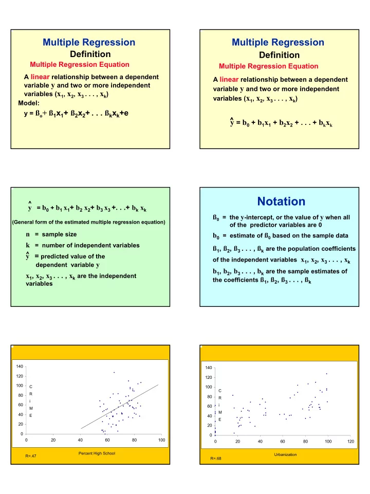
20 40 60 80 100 120 140 20 40 60 80 100 Percent High School C R i M E R=.47 20 40 60 80 100 120 140 20 40 60 80 100 120 C R i M E Urbanization R=.68

slide-2
SLIDE 2

52462 66 Corrected Total 433.28847 27730 64 Error <.0001 28.54 12366 24732 2 Model Pr > F F Value Mean Square Sum of Squares DF Source Analysis of Variance

Overall Regression Analysis: A Test of the Multiple R

39.72213 Coeff Var 0.4549 Adj R-Sq 52.40299 Dependent Mean 0.4714 R-Square 20.81558 Root MSE

(R=.686)

<.0001 5.54 0.12321 0.68250 1 Urb 0.2214

  • 1.23

0.47246

  • 0.58338

1 hs 0.0411 2.08 28.36531 59.11807 1 Intercept Pr > |t| t Value Standard Error Parameter Estimate DF Variable Parameter Estimates

Notice that the slope of hs is negative

<.0001 4.26 0.34908 1.48598 1 hs 0.0415

  • 2.08

24.45065

  • 50.85690

1 Intercept Pr > |t| t Value Standard Error Parameter Estimate DF Variable Parameter Estimates

When hs is by itself the slope is positive

1.00000 0.79072 <.0001 0.73070 <.0001 0.67737 <.0001 Urb 0.79072 <.0001 1.00000 0.79262 <.0001 0.46691 <.0001 hs 0.73070 <.0001 0.79262 <.0001 1.00000 0.43375 0.0002 incom 0.67737 <.0001 0.46691 <.0001 0.43375 0.0002 1.00000 crate Urb hs incom crate Pearson Correlation Coefficients, N = 67 Prob > |r| under H0: Rho=0

slide-3
SLIDE 3

Multiple Regression SAS Setup

  • proc corr; run;
  • proc reg; model crate= hs Urb;
  • plot crate*hs;run;
  • proc reg; model crate= hs;run;

Adjusted R2

Multiple coefficient of determination

a measure of how well the multiple regression equation fits the sample data

Adjusted coefficient of determination

the multiple coefficient of determination

R2 modified to account for the number of

variables and the sample size

Definitions

Adjusted R

2

Adjusted R

2

Adjusted R

2 = 1 -

(n - 1)

[n - (k + 1)] (1 - R

2)

Adjusted R

2

Adjusted R

2 = 1 -

(n - 1)

[n - (k + 1)] (1 - R

2)

where n = sample size

k = number of independent (x) variables

Including the Three Variables

Analysis of Variance Source

DF

Sum of Squares Mean Square F Value Pr > F Model 3 24804 8268.16424 18.83 <.0001 Error 63 27658 439.00995 Corrected Total 66 52462

slide-4
SLIDE 4

Overall Test

Root MSE 20.95256 R-Square 0.4728 Dependent Mean 52.40299 Adj R-Sq 0.4477 Coeff Var 39.98353

Tests of Hypotheses

  • Overall test:

Null: All of the population regression weights are zero. Alternative: Not all are zero

The overall F Test

) 1 /( ) 1 ( /

2 2 1 ,

− − − =

− −

k n R k R F

k n k

Parameter Estimates Variable DF Parameter Estimate Standard Error t Value Pr > |t| Intercept 1 59.71473 28.58953 2.09 0.0408 incom 1

  • 0.38309

0.94053

  • 0.41

0.6852 hs 1

  • 0.46729

0.55443

  • 0.84

0.4025 Urb 1 0.69715 0.12913 5.40 <.0001

Individual Tests

  • Test for b1:

Y = bo + b1x1 + b2x 2 + b3x3 + e Y = bo + b2x 2 + b3x3 + e

  • Test for b2:

Y = bo + b1x1 + b2x 2 + b3x3 + e Y = bo + b1x1 + b3x3 + e

  • Test for b3:

Y = bo + b1x1 + b2x 2 + b3x3 + e Y = bo + b1x1 + b2x 2 + e

F Test for Restricted Models

) 1 /( ) 1 ( ) /( ) (

2 2 2 1 ,

− − − − − =

− − −

k n R g k R R F

f r f k n g k

slide-5
SLIDE 5

More on SAS

  • Model options:

Model y = x1 x2 / R partial p stb; R– residual analysis Partial– partial regression scatter plot P– predicted values Stb– standardized regression weights

Standardized Regression Weights

        =

y x i i

S S b b

i

*

Generally, the standardized regression weights fall between 1 and –1. However, they can larger than one (or less than –1).

Obtaining the Standardized Regression Weights

  • Model Statement

– Model crate = incom hs urb /stb;

Parameter Estimates Variable DF Parameter Estimate Standard Error t Value Pr > |t| Standardized Estimate Intercept 1 59.71473 28.58953 2.09 0.0408 incom 1

  • 0.38309

0.94053

  • 0.41

0.6852

  • 0.06363

hs 1

  • 0.46729

0.55443

  • 0.84

0.4025

  • 0.14683

Urb 1 0.69715 0.12913 5.40 <.0001 0.83996

Partial Regression Plots

  • Plot of two residuals
  • The regression line in this plot corresponds

to the regression weight in the overall model.

  • Model Statement

/ partial

„ƒˆƒƒƒƒƒˆƒƒƒƒƒˆƒƒƒƒƒˆƒƒƒƒƒˆƒƒƒƒƒˆƒƒƒƒƒˆƒƒƒƒƒˆƒƒƒƒƒˆƒƒƒƒƒˆƒƒƒƒƒˆƒƒƒƒƒˆƒƒƒƒƒˆƒƒƒƒƒˆƒƒƒƒƒˆƒƒ† crate ‚ ‚ ‚ ‚ ‚ ‚ ‚ ‚ ‚ ‚ 60 ˆ ˆ ‚ ‚ ‚ ‚ ‚ 1 ‚ ‚ 1 ‚ ‚ ‚ 40 ˆ 1 ˆ ‚ 1 1 ‚ ‚ 1 ‚ ‚ ‚ ‚ 1 1 1 ‚ ‚ 1 ‚ 20 ˆ 1 1 1 ˆ ‚ 1 1 1 11 1 1 ‚ ‚ 1 1 1 ‚ ‚ 1 1 1 ‚ ‚ ‚ ‚ 1 ‚ 0 ˆ 1 1 ˆ ‚ 1 1 1 ‚ ‚ 1 1 1 1 ‚ ‚ 1 1 2 ‚ ‚ 1 1 1 1 1 11 1 1 ‚ ‚ 1 1 1 1 1 1 1 ‚

  • 20 ˆ

2 1 ˆ ‚ 2 1 1 ‚ ‚ 1 ‚ ‚ ‚ ‚ 1 1 ‚ ‚ 1 ‚

  • 40 ˆ

ˆ ‚ ‚ ‚ ‚ ‚ ‚ ‚ ‚ ‚ ‚ ŠƒˆƒƒƒƒƒˆƒƒƒƒƒˆƒƒƒƒƒˆƒƒƒƒƒˆƒƒƒƒƒˆƒƒƒƒƒˆƒƒƒƒƒˆƒƒƒƒƒˆƒƒƒƒƒˆƒƒƒƒƒˆƒƒƒƒƒˆƒƒƒƒƒˆƒƒƒƒƒˆƒƒƒƒƒˆƒƒŒ

  • 14 -12 -10 -8 -6 -4 -2 0 2 4 6 8 10 12 14

hs

Hs-b1(inc)-b2(urb) Crate-b1(inc)-b2(urb)

slide-6
SLIDE 6

„ƒˆƒƒƒƒƒƒˆƒƒƒƒƒƒˆƒƒƒƒƒƒˆƒƒƒƒƒƒˆƒƒƒƒƒƒˆƒƒƒƒƒƒˆƒƒƒƒƒƒˆƒƒƒƒƒƒˆƒƒƒƒƒƒˆƒƒƒƒƒƒˆƒƒƒƒƒƒˆƒƒƒƒƒƒˆƒƒ† crate ‚ ‚ ‚ ‚ ‚ ‚ 80 ˆ ˆ ‚ 1 ‚ ‚ ‚ ‚ ‚ ‚ ‚ 60 ˆ ˆ ‚ ‚ ‚ ‚ ‚ 1 ‚ ‚ ‚ 40 ˆ 1 1 ˆ ‚ 1 1 1 ‚ ‚ 11 ‚ ‚ 1 1 ‚ ‚ 1 1 ‚ 20 ˆ 1 1 1 1 1 1 ˆ ‚ 1 ‚ ‚ 1 1 ‚ ‚ 1 1 1 1 ‚ ‚ 1 1 1 1 1 ‚ 0 ˆ ˆ ‚ 1 1 1 1 1 ‚ ‚ 1 1 1 1 11 ‚ ‚ 1 1 ‚ ‚ 1 1 1 1 1 ‚

  • 20 ˆ

1 1 ˆ ‚ 1 1 1 ‚ ‚ 1 1 12 1 1 1 ‚ ‚ 1 1 ‚ ‚ 1 1 ‚

  • 40 ˆ

ˆ ‚ 1 ‚ ‚ ‚ ‚ ‚ ‚ ‚

  • 60 ˆ

ˆ ‚ ‚ ‚ ‚ ŠƒˆƒƒƒƒƒƒˆƒƒƒƒƒƒˆƒƒƒƒƒƒˆƒƒƒƒƒƒˆƒƒƒƒƒƒˆƒƒƒƒƒƒˆƒƒƒƒƒƒˆƒƒƒƒƒƒˆƒƒƒƒƒƒˆƒƒƒƒƒƒˆƒƒƒƒƒƒˆƒƒƒƒƒƒˆƒƒŒ

  • 60 -50 -40 -30 -20 -10 0 10 20 30 40 50 60

Urb

Crate-b1(inc)-b2(hs) Urb-b1(inc)-b2(hs)

Interaction of two Variables

  • Just as in ANOVA we can have interaction effects

in a multiple regression analysis.

  • For quantitative variables, interaction is present

when the relationship between the explanatory variable and the response changes as the levels of another variable changes.

  • Consider crime rate as a function of hs and urb. If

the relationship (slope) between crime rate and urb changes as hs changes, we have an interaction between urb and hs.

Testing for an Interaction Effect

  • We test for interaction effect by comparing

a model with interaction to a model without interaction:

Y = βo + β1x1 + β2x2 + β3 (x1*x2) + e Y = βo + β1x1 + β2x2 + e

SAS Setup for Interaction

  • Create a the product variable in the data

statement:

– Data new; input y x z; xz=x*z; cards; – Model y = x z xz;

Root MSE 20.82583 R-Square 0.4792 Dependent Mean 52.40299 Adj R-Sq 0.4544 Coeff Var 39.74168

Model crate= hs urb hs*urb (Looking for an interaction)

Parameter Estimates Variable DF Parameter Estimate Standard Error t Value Pr > |t| Intercept 1 19.31754 49.95871 0.39 0.7003 hs 1 0.03396 0.79381 0.04 0.9660 Urb 1 1.51431 0.86809 1.74 0.0860 hsurb 1

  • 0.01205

0.01245

  • 0.97

0.3367

Testing the Interaction

slide-7
SLIDE 7

SAS Setup for Interaction

data crime; input crate incom hs Urb; hsurb= hs*urb;cards; 104 22.1 82.7 73.2 proc reg; model crate= hs Urb hsurb; run;

Assessing The Fit of the Model

Looking further at residuals Residual Plots in Regression

Plot of yresid*hs. Legend: A = 1 obs, B = 2 obs, etc. ‚ ‚ 60 ˆ ‚ ‚ ‚ A ‚ ‚ ‚ 40 ˆ A A A ‚ A ‚ A ‚ ‚ A ‚ A A R ‚ A A e 20 ˆ A A s ‚ A A A A i ‚ A AA AA d ‚ A A u ‚ A a ‚ A l ‚ A 0 ˆ B ‚ A A ‚ A A A ‚ A A A A A A ‚ A A A A ‚ A A A A A A A ‚ A A A A A

  • 20 ˆ

A A A A ‚ A ‚ A A A ‚ ‚ A ‚ A A ‚

  • 40 ˆ

‚ Šƒƒˆƒƒƒƒƒƒƒƒƒƒƒˆƒƒƒƒƒƒƒƒƒƒƒˆƒƒƒƒƒƒƒƒƒƒƒˆƒƒƒƒƒƒƒƒƒƒƒˆƒƒƒƒƒƒƒƒƒƒƒˆƒƒƒƒƒƒƒƒƒƒƒˆƒƒƒƒƒƒƒƒƒƒƒˆƒƒ 50 55 60 65 70 75 80 85 hs

Residual by hs

Plot of yresid*Urb. Legend: A = 1 obs, B = 2 obs, etc. ‚ ‚ 60 ˆ ‚ ‚ ‚ A ‚ ‚ ‚ 40 ˆ A A A ‚ A ‚ A ‚ ‚ A ‚ A A R ‚ B e 20 ˆ A A s ‚ A A A A i ‚ A A A B d ‚ A A u ‚ A a ‚ A l ‚ A 0 ˆ A A ‚ A A ‚ A A A ‚ A A A A A A ‚ AAA A ‚ A AA A A A A ‚ B A A A

  • 20 ˆ

A A AA ‚ A ‚ A A A ‚ ‚ A ‚ A A ‚

  • 40 ˆ

‚ Šƒƒˆƒƒƒƒƒƒƒƒƒƒƒƒƒˆƒƒƒƒƒƒƒƒƒƒƒƒƒˆƒƒƒƒƒƒƒƒƒƒƒƒƒˆƒƒƒƒƒƒƒƒƒƒƒƒƒˆƒƒƒƒƒƒƒƒƒƒƒƒƒˆƒƒ 0 20 40 60 80 100 Urb

Residual by Urb

Plot of yresid*incom. Legend: A = 1 obs, B = 2 obs, etc. ‚ ‚ 60 ˆ ‚ ‚ ‚ A ‚ ‚ ‚ 40 ˆ A AA ‚ A ‚ A ‚ ‚ A ‚ A A R ‚ A A e 20 ˆ A A s ‚ A A A A i ‚ A A A A A d ‚ A A u ‚ A a ‚ A l ‚ A 0 ˆ A A ‚ A A ‚ A A A ‚ A A A A A A ‚ B A A ‚ A A A A A A A ‚ A AA A A

  • 20 ˆ

AA B ‚ A ‚ A A A ‚ ‚ A ‚ A A ‚

  • 40 ˆ

‚ Šƒƒˆƒƒƒƒƒƒƒƒˆƒƒƒƒƒƒƒƒˆƒƒƒƒƒƒƒƒˆƒƒƒƒƒƒƒƒˆƒƒƒƒƒƒƒƒˆƒƒƒƒƒƒƒƒˆƒƒƒƒƒƒƒƒˆƒƒƒƒƒƒƒƒˆƒƒƒƒƒƒƒƒˆƒƒ 15.0 17.5 20.0 22.5 25.0 27.5 30.0 32.5 35.0 37.5 incom

Residual by income

slide-8
SLIDE 8

SAS Setup

  • proc reg;
  • model crate= incom hs Urb;
  • output out=new p=yhat r=yresid;
  • proc plot data=new;
  • plot yresid*hs;
  • plot yresid*urb;
  • plot yresid*incom;run;

Assumptions

  • Linearity– the relationship between the

dependent variable and independent variables is linear.

  • Normality– y is independently normally

distributed

Independently distributed random errors with a mean of zero.

  • Homoskedasticity– the conditional

variances of y given x are all equal.

Investigating Multicollinearty

  • SAS Model Statement:
  • model crate= incom hs Urb / vif

collin;

  • When the explanatory variables are

highly correlated (multicollinearity) the standard errors of the regression weights tend to get very large.

Collinearity Diagnostics Number Eigenvalue Condition Index Proportion of Variation Intercept incom hs Urb 1 3.78327 1.00000 0.00053670 0.00082225 0.00029978 0.00648 2 0.20397 4.30678 0.00735 0.00127 0.00107 0.39725 3 0.00983 19.61619 0.22868 0.81261 0.00944 0.29914 4 0.00293 35.92811 0.76343 0.18530 0.98919 0.29712

Using the Multicollinearity Indices

  • Look for conditioned indices larger than 30
  • If an index is large than 30, identify

variables with proportion indices larger than .90

– Proportion of variance in each coefficient attributable to the condition index.

Parameter Estimates Variable DF Parameter Estimate Standard Error t Value Pr > |t| Variance Inflation Intercept 1 59.71473 28.58953 2.09 0.0408 incom 1

  • 0.38309

0.94053

  • 0.41

0.6852 2.91618 hs 1

  • 0.46729

0.55443

  • 0.84

0.4025 3.62675 Urb 1 0.69715 0.12913 5.40 <.0001 2.89274

slide-9
SLIDE 9

Variance Inflation Factor (VIF)

VIF VIF R rest

i

1

2 .

− =

VIF– the variance of the weight is inflated by this quantity.

Root MSE 4.72386 R-Square 0.7243 Dependent Mean 69.48955 Adj R-Sq 0.7157 Coeff Var 6.79794

Model: hs = income urbanization

Collinearity Diagnostics Number Eigenvalue Condition Index Proportion of Variation Intercept incom Urb 1 2.80034 1.00000 0.00293 0.00203 0.01645 2 0.19004 3.83868 0.03655 0.00499 0.50952 3 0.00962 17.06408 0.96052 0.99299 0.47402

Test that a subset of regression weights are equal to zero

  • SAS Test Statement:

proc reg; model crate= incom hs urb; test incom=0, hs=0; run; Or, test incom, hs;

Results from the Joint test βhs=βincom=0

Test 1 Results for Dependent Variable crate Source DF Mean Square F Value Pr > F Numerator 2 366.72473 0.84 0.4385 Denominator 63 439.00995

Partial Correlations

  • In a partial correlation a variable is partial
  • ut of both variables

rx1x2 . x3

2 23 . 1 2 3 . 1 2 23 . 1 2 3 . 12

1 R R R r − − =

slide-10
SLIDE 10

y1 x z y2 x z

Ry1y2.xz

„ƒˆƒƒƒƒƒƒˆƒƒƒƒƒƒˆƒƒƒƒƒƒˆƒƒƒƒƒƒˆƒƒƒƒƒƒˆƒƒƒƒƒƒˆƒƒƒƒƒƒˆƒƒƒƒƒƒˆƒƒƒƒƒƒˆƒƒƒƒƒƒˆƒƒƒƒƒƒˆƒƒƒƒƒƒˆƒƒ† crate ‚ ‚ ‚ ‚ ‚ ‚ 80 ˆ ˆ ‚ 1 ‚ ‚ ‚ ‚ ‚ ‚ ‚ 60 ˆ ˆ ‚ ‚ ‚ ‚ ‚ 1 ‚ ‚ ‚ 40 ˆ 1 1 ˆ ‚ 1 1 1 ‚ ‚ 11 ‚ ‚ 1 1 ‚ ‚ 1 1 ‚ 20 ˆ 1 1 1 1 1 1 ˆ ‚ 1 ‚ ‚ 1 1 ‚ ‚ 1 1 1 1 ‚ ‚ 1 1 1 1 1 ‚ 0 ˆ ˆ ‚ 1 1 1 1 1 ‚ ‚ 1 1 1 1 11 ‚ ‚ 1 1 ‚ ‚ 1 1 1 1 1 ‚

  • 20 ˆ

1 1 ˆ ‚ 1 1 1 ‚ ‚ 1 1 12 1 1 1 ‚ ‚ 1 1 ‚ ‚ 1 1 ‚

  • 40 ˆ

ˆ ‚ 1 ‚ ‚ ‚ ‚ ‚ ‚ ‚

  • 60 ˆ

ˆ ‚ ‚ ‚ ‚ ŠƒˆƒƒƒƒƒƒˆƒƒƒƒƒƒˆƒƒƒƒƒƒˆƒƒƒƒƒƒˆƒƒƒƒƒƒˆƒƒƒƒƒƒˆƒƒƒƒƒƒˆƒƒƒƒƒƒˆƒƒƒƒƒƒˆƒƒƒƒƒƒˆƒƒƒƒƒƒˆƒƒƒƒƒƒˆƒƒŒ

  • 60 -50 -40 -30 -20 -10 0 10 20 30 40 50 60

Urb

Crate-b1(inc)-b2(hs) Urb-b1(inc)-b2(hs)

Semipartial Correlations

  • The variable is partial out from only one of

the variables. The squared semipartial correlation is given by

2 3 . 1 2 23 . 1 2 ) 3 . 2 ( 1

R R r − =

Relationship between Semipartials and the Multiple R2

2 ) 123 . 4 ( 2 ) 12 . 3 ( 2 ) 1 . 2 ( 2 1 . 2 1234 . y y y y y

r r r r R + + + =

Finding the Best Multiple Regression Equation

  • 1. Use common sense and practical considerations to

include or exclude variables and always plot the data.

  • 2. Instead of including almost every available variable,

include relatively few independent (x) variables, weeding out independent variables that don’t have an effect on the dependent variable, remember collinearity.

  • 3. Select an equation having a value of adjusted R2 with this

property: If an additional independent variable is included, the value of adjusted R2 does not increase by a substantial amount. 4. For a given number of independent (x) variables, select the equation with the largest value of adjusted R2. 5. You want overall significance with all of the regression weights being significant also.