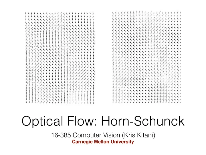
Optical Flow: Horn-Schunck 16-385 Computer Vision (Kris Kitani) - - PowerPoint PPT Presentation

Optical Flow: Horn-Schunck

16-385 Computer Vision (Kris Kitani)

Carnegie Mellon University

Horn-Schunck Optical Flow (1981) Lucas-Kanade Optical Flow (1981) ‘constant’ flow

(flow is constant for all pixels)

‘smooth’ flow

(flow can vary from pixel to pixel)

brightness constancy method of differences global method (dense) local method (sparse) small motion

Optical Flow

(Problem definition)

Estimate the motion (flow) between these two consecutive images I(x, y, t) I(x, y, t0) How is this different from estimating a 2D transform?

Key Assumptions

(unique to optical flow)

Color Constancy

(Brightness constancy for intensity images)

Small Motion

(pixels only move a little bit)

Implication: allows for pixel to pixel comparison (not image features) Implication: linearization of the brightness constancy constraint

Approach

I(x, y, t) I(x, y, t0)

Look for nearby pixels with the same color

(small motion) (color constancy)

Brightness constancy

I(x, y, t)

(x, y) (x + uδt, y + vδt) (x, y)

(u, v) (δx, δy) = (uδt, vδt)

Optical flow (velocities): Displacement:

I(x + uδt, y + vδt, t + δt) = I(x, y, t)

I(x, y, t + δt)

For a really small time step…

Optical Flow Constraint equation

I(x + uδt, y + vδt, t + δt) = I(x, y, t)

I(x, y, t) + ∂I ∂xδx + ∂I ∂y δy + ∂I ∂t δt = I(x, y, t)

Ixu + Iyv + It = 0

∂I ∂x dx dt + ∂I ∂y dy dt + ∂I ∂t = 0

Ixu + Iyv + It = 0

u

v

Solution lies on a straight line The solution cannot be determined uniquely with a single constraint (a single pixel)

Where can we get an additional constraint?

Horn-Schunck Optical Flow (1981) Lucas-Kanade Optical Flow (1981) ‘constant’ flow

(flow is constant for all pixels)

‘smooth’ flow

(flow is smooth from pixel to pixel)

brightness constancy method of differences global method local method small motion

Smoothness

most objects in the world are rigid or deform elastically moving together coherently we expect optical flow fields to be smooth

Key idea

(of Horn-Schunck optical flow)

Enforce brightness constancy Enforce smooth flow field to compute optical flow

Key idea

(of Horn-Schunck optical flow)

Enforce brightness constancy Enforce smooth flow field to compute optical flow

Enforce 
 brightness constancy

Ixu + Iyv + It = 0

min

u,v

 Ixuij + Iyvij + It 2

For every pixel,

Ixu + Iyv + It = 0

min

u,v

 Ixuij + Iyvij + It 2

For every pixel,

lazy notation for Ix(i, j)

Enforce 
 brightness constancy

Ix

Iy

changes these displacement of object

u v

changes these

It

+ =

Find the optical flow such that it satisfies:

Key idea

(of Horn-Schunck optical flow)

Enforce brightness constancy Enforce smooth flow field to compute optical flow

Enforce smooth flow field

uij

ui+1,j ui−1,j

ui,j+1 ui,j−1

min u (ui,j − ui+1,j)2

u-component of flow

Which flow field optimizes the objective?

X

ij

(uij − ui+1,j)2 X

ij

(uij − ui+1,j)2

?

min u (ui,j − ui+1,j)2

small big Which flow field optimizes the objective?

min u (ui,j − ui+1,j)2

Key idea

(of Horn-Schunck optical flow)

Enforce brightness constancy Enforce smooth flow field to compute optical flow bringing it all together…

Horn-Schunck optical flow

min u,v X

i,j

⇢ Es(i, j) + λEd(i, j)

• smoothness

brightness constancy weight

HS optical flow objective function

Brightness constancy Smoothness

(uij − ui+1,j)

ij

i, j + 1

i + 1, j

ij

i, j + 1

i + 1, j i − 1, j i, j − 1 i − 1, j i, j − 1

(uij − ui,j+1)

ij

i, j + 1 i + 1, j

ij

i, j + 1

i + 1, j i − 1, j i, j − 1 i − 1, j i, j − 1

(vij − vi+1,j) (vij − vi,j+1)

Ed(i, j) =  Ixuij + Iyvij + It 2

Es(i, j) = 1 4  (uij − ui+1,j)2 + (uij − ui,j+1)2 + (vij − vi+1,j)2 + (vij − vi,j+1)2

• why not all four neighbors?

How do we solve this minimization problem?

min u,v X

i,j

⇢ Es(i, j) + λEd(i, j)

Compute partial derivative, derive update equations

(gradient decent!)

min u,v X

i,j

⇢ Es(i, j) + λEd(i, j)

• How do we solve this

minimization problem?

Compute the partial derivatives of this huge sum!

X

ij

( 1 4  (uij − ui+1,j)2 + (uij − ui,j+1)2 + (vij − vi+1,j)2 + (vij − vi,j+1)2

• + λ

 Ixuij + Iyvij + It 2)

smoothness term brightness constancy

Compute the partial derivatives of this huge sum!

X

ij

( 1 4  (uij − ui+1,j)2 + (uij − ui,j+1)2 + (vij − vi+1,j)2 + (vij − vi,j+1)2

• + λ

 Ixuij + Iyvij + It 2)

∂E ∂ukl =

it’s not so bad… how many u terms depend on k and l?

Compute the partial derivatives of this huge sum!

X

ij

( 1 4  (uij − ui+1,j)2 + (uij − ui,j+1)2 + (vij − vi+1,j)2 + (vij − vi,j+1)2

• + λ

 Ixuij + Iyvij + It 2)

∂E ∂ukl =

it’s not so bad… how many u terms depend on k and l?

ONE from brightness constancy FOUR from smoothness

Compute the partial derivatives of this huge sum!

X

ij

( 1 4  (uij − ui+1,j)2 + (uij − ui,j+1)2 + (vij − vi+1,j)2 + (vij − vi,j+1)2

• + λ

 Ixuij + Iyvij + It 2)

∂E ∂ukl = 2(ukl − ¯ ukl) + 2λ(Ixukl + Iyvkl + It)Ix

it’s not so bad… how many u terms depend on k and l?

ONE from brightness constancy FOUR from smoothness

Compute the partial derivatives of this huge sum!

X

ij

( 1 4  (uij − ui+1,j)2 + (uij − ui,j+1)2 + (vij − vi+1,j)2 + (vij − vi,j+1)2

• + λ

 Ixuij + Iyvij + It 2)

(uij − ui+1,j)

ij

i, j + 1 i + 1, j

i − 1, j i, j − 1

(u2

ij − 2uijui+1,j + u2 i+1,j)

(u2

ij − 2uijui,j+1 + u2 i,j+1)

(variable will appear four times in sum)

Compute the partial derivatives of this huge sum!

X

ij

( 1 4  (uij − ui+1,j)2 + (uij − ui,j+1)2 + (vij − vi+1,j)2 + (vij − vi,j+1)2

• + λ

 Ixuij + Iyvij + It 2)

(uij − ui+1,j)

ij

i, j + 1 i + 1, j

i − 1, j i, j − 1

∂E ∂vkl = 2(vkl − ¯ vkl) + 2λ(Ixukl + Iyvkl + It)Iy ∂E ∂ukl = 2(ukl − ¯ ukl) + 2λ(Ixukl + Iyvkl + It)Ix

¯ uij = 1 4 ⇢ ui+1,j + ui−1,j + ui,j+1 + ui,j−1

• short hand for

local average

(u2

ij − 2uijui+1,j + u2 i+1,j)

(u2

ij − 2uijui,j+1 + u2 i,j+1)

(variable will appear four times in sum)

∂E ∂vkl = 2(vkl − ¯ vkl) + 2λ(Ixukl + Iyvkl + It)Iy ∂E ∂ukl = 2(ukl − ¯ ukl) + 2λ(Ixukl + Iyvkl + It)Ix Where are the extrema of E?

∂E ∂vkl = 2(vkl − ¯ vkl) + 2λ(Ixukl + Iyvkl + It)Iy ∂E ∂ukl = 2(ukl − ¯ ukl) + 2λ(Ixukl + Iyvkl + It)Ix Where are the extrema of E?

(set derivatives to zero and solve for unknowns u and v)

λIxIyukl + (1 + λI2

y)vkl = ¯

vkl − λIyIt (1 + λI2

x)ukl + λIxIyvkl = ¯

ukl − λIxIt

∂E ∂vkl = 2(vkl − ¯ vkl) + 2λ(Ixukl + Iyvkl + It)Iy ∂E ∂ukl = 2(ukl − ¯ ukl) + 2λ(Ixukl + Iyvkl + It)Ix Where are the extrema of E?

(set derivatives to zero and solve for unknowns u and v)

Ax = b

how do you solve this?

λIxIyukl + (1 + λI2

y)vkl = ¯

vkl − λIyIt (1 + λI2

x)ukl + λIxIyvkl = ¯

ukl − λIxIt

this is a linear system

• k, take a step back, why are we doing all this math?

X

ij

( 1 4  (uij − ui+1,j)2 + (uij − ui,j+1)2 + (vij − vi+1,j)2 + (vij − vi,j+1)2

• + λ

 Ixuij + Iyvij + It 2)

We are solving for the optical flow (u,v) given two constraints

smoothness brightness constancy

We need the math to minimize this (back to the math)

∂E ∂vkl = 2(vkl − ¯ vkl) + 2λ(Ixukl + Iyvkl + It)Iy ∂E ∂ukl = 2(ukl − ¯ ukl) + 2λ(Ixukl + Iyvkl + It)Ix Where are the extrema of E?

(set derivatives to zero and solve for unknowns u and v)

Ax = b

how do you solve this?

λIxIyukl + (1 + λI2

y)vkl = ¯

vkl − λIyIt (1 + λI2

x)ukl + λIxIyvkl = ¯

ukl − λIxIt

Partial derivatives of Horn-Schunck objective function E:

x = A−1b = adjA det Ab

Recall λIxIyukl + (1 + λI2

y)vkl = ¯

vkl − λIyIt (1 + λI2

x)ukl + λIxIyvkl = ¯

ukl − λIxIt

x = A−1b = adjA det Ab

Recall

(det A)

λIxIyukl + (1 + λI2

y)vkl = ¯

vkl − λIyIt (1 + λI2

x)ukl + λIxIyvkl = ¯

ukl − λIxIt Same as the linear system: {1 + λ(I2

x + I2 y)}ukl = (1 + λI2 x)¯

ukl − λIxIy¯ vkl − λIxIt {1 + λ(I2

x + I2 y)}vkl = (1 + λI2 y)¯

vkl − λIxIy¯ ukl − λIyIt

(det A)

Rearrange to get update equations:

new value

• ld

average

{1 + λ(I2

x + I2 y)}ukl = (1 + λI2 x)¯

ukl − λIxIy¯ vkl − λIxIt {1 + λ(I2

x + I2 y)}vkl = (1 + λI2 y)¯

vkl − λIxIy¯ ukl − λIyIt

ˆ ukl = ¯ ukl − Ix¯ ukl + Iy¯ vkl + It λ−1 + I2

x + I2 y

Ix

ˆ vkl = ¯ vkl − Ix¯ ukl + Iy¯ vkl + It λ−1 + I2

x + I2 y

Iy

new value

• ld

average

ˆ ukl = ¯ ukl − Ix¯ ukl + Iy¯ vkl + It λ−1 + I2

x + I2 y

Ix

ˆ vkl = ¯ vkl − Ix¯ ukl + Iy¯ vkl + It λ−1 + I2

x + I2 y

Iy

When lambda is small (lambda inverse is big)…

min u,v X

i,j

⇢ Es(i, j) + λEd(i, j)

• Recall:

new value

• ld

average

ˆ ukl = ¯ ukl − Ix¯ ukl + Iy¯ vkl + It λ−1 + I2

x + I2 y

Ix

ˆ vkl = ¯ vkl − Ix¯ ukl + Iy¯ vkl + It λ−1 + I2

x + I2 y

Iy

When lambda is small (lambda inverse is big)…

goes to zero goes to zero

min u,v X

i,j

⇢ Es(i, j) + λEd(i, j)

• Recall:

new value

• ld

average

ˆ ukl = ¯ ukl − Ix¯ ukl + Iy¯ vkl + It λ−1 + I2

x + I2 y

Ix

ˆ vkl = ¯ vkl − Ix¯ ukl + Iy¯ vkl + It λ−1 + I2

x + I2 y

Iy

When lambda is small (lambda inverse is big)…

goes to zero goes to zero

…we only care about smoothness.

min u,v X

i,j

⇢ Es(i, j) + λEd(i, j)

• Recall:

• k, take a step back, why did we do all this math?

X

ij

( 1 4  (uij − ui+1,j)2 + (uij − ui,j+1)2 + (vij − vi+1,j)2 + (vij − vi,j+1)2

• + λ

 Ixuij + Iyvij + It 2)

We are solving for the optical flow (u,v) given two constraints

smoothness brightness constancy

We needed the math to minimize this (now to the algorithm)

Horn-Schunck 
 Optical Flow Algorithm

• 1. Precompute image gradients
• 2. Precompute temporal gradients
• 3. Initialize flow field
• 4. While not converged



 Compute flow field updates for each pixel:

Ix Iy It

u = 0 v = 0 ˆ ukl = ¯ ukl − Ix¯ ukl + Iy¯ vkl + It λ−1 + I2

x + I2 y

Ix ˆ vkl = ¯ vkl − Ix¯ ukl + Iy¯ vkl + It λ−1 + I2

x + I2 y

Iy Just 8 lines of code!