Outline International Conference on Computational Methods (ICCM - - PDF document

SLIDE 1

1 Numerical Simulations in the SILC Matrix Computation Framework

Tamito KAJIYAMA (JST / University of Tokyo, Japan) Akira NUKADA (JST / University of Tokyo, Japan) Reiji SUDA (University of Tokyo / JST, Japan) Hidehiko HASEGAWA (University of Tsukuba, Japan) Akira NISHIDA (Chuo University / JST, Japan)

International Conference on Computational Methods (ICCM 2007) April 4-6, 2007, Hiroshima, Japan

Outline

• The SILC matrix computation framework

– Easy-to-use interface for matrix computation libraries

• Proposal of two application modes for SILC
• Two applications in numerical simulations

– Cloth simulation in C – MPS-based simulation in Java

• Experimental results
• Concluding remarks

Overview of the SILC framework

• Simple Interface for Library Collections

– Independent of libraries, environments & languages – Easy to use

• Three steps to use libraries

– Depositing data (matrices, vectors, etc.) to a server – Making requests for computation by means of mathematical expressions – Fetching the results of computation if necessary

User program (client) SILC server

Matrix computation libraries

Depositing data Fetching results "x = A＼b"

5.0 4.0 3.0 2.0 1.0 0.2 0.4 0.6 0.8 1 x Time (in seconds)

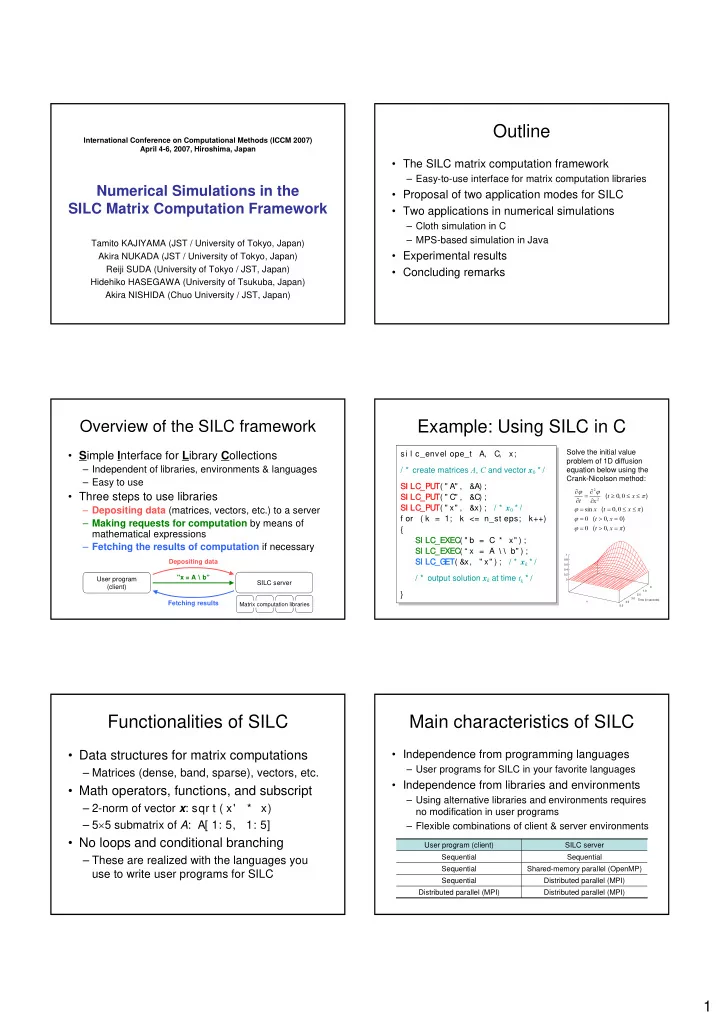
Example: Using SILC in C

) , ( ) , ( ) , ( ) , ( π x t x t π x t x x t x t = > = = > = ≤ ≤ = = ≤ ≤ ≥ ∂ ∂ = ∂ ∂ sin

2 2

ϕ ϕ ϕ π ϕ ϕ

si l c_envel ope_t A, C, x; / * create matrices A, C and vector x0 * / SI LC_PUT SI LC_PUT( " A" , &A) ; SI LC_PUT SI LC_PUT( " C" , &C) ; SI LC_PUT SI LC_PUT( " x" , &x) ; / * x0 * / f or ( k = 1; k <= n_st eps; k++) { SI LC_E SI LC_EXEC XEC( " b = C * x" ) ; SI LC_E SI LC_EXEC XEC( “ x = A ∖ ∖ b" ) ; SI LC_G SI LC_G ET ET( &x, " x" ) ; / * xk * / / * output solution xk at time tk * / } si l c_envel ope_t A, C, x; / * create matrices A, C and vector x0 * / SI LC_PUT SI LC_PUT( " A" , &A) ; SI LC_PUT SI LC_PUT( " C" , &C) ; SI LC_PUT SI LC_PUT( " x" , &x) ; / * x0 * / f or ( k = 1; k <= n_st eps; k++) { SI LC_E SI LC_EXEC XEC( " b = C * x" ) ; SI LC_E SI LC_EXEC XEC( “ x = A ∖ ∖ b" ) ; SI LC_G SI LC_G ET ET( &x, " x" ) ; / * xk * / / * output solution xk at time tk * / }

Solve the initial value problem of 1D diffusion equation below using the Crank-Nicolson method:

Functionalities of SILC

• Data structures for matrix computations

– Matrices (dense, band, sparse), vectors, etc.

• Math operators, functions, and subscript

– 2-norm of vector x: sqr t ( x' * x) – 5×5 submatrix of A: A[ 1: 5, 1: 5]

• No loops and conditional branching

– These are realized with the languages you use to write user programs for SILC

Main characteristics of SILC

• Independence from programming languages

– User programs for SILC in your favorite languages

• Independence from libraries and environments

– Using alternative libraries and environments requires no modification in user programs – Flexible combinations of client & server environments

Distributed parallel (MPI) Distributed parallel (MPI) Distributed parallel (MPI) Sequential Shared-memory parallel (OpenMP) Sequential Sequential Sequential SILC server User program (client)

SLIDE 2

2

Proposal of two application modes

• Limited application mode

– Use SILC only in the most time-consuming, computationally intensive part of a program

• Comprehensive application mode

– Move all relevant data to a SILC server, and implement overall simulations using SILC's mathematical expressions Abbreviations:

• LTD for the limited application mode
• CMP for the comprehensive application mode

Limited application mode

• Pros

– Easy to apply (especially to existing user programs)

• Cons

– Smaller data size due to a limited amount of main memory in client environments – Frequent data communications (larger overheads)

Use SILC only in the most time-consuming, computationally intensive part of a program Use SILC only in the most time-consuming, computationally intensive part of a program

Application #1

• Time-dependent simulation of cloth motion

– Mass-spring model – Implicit Euler method – Solving a sparse linear system is necessary for each time step

• Original code

– Sequential program in C – Linear solver: CG method – Visualization: OpenGL

Original code

• 1. Calculate force f and its derivatives ∂f /∂x and

∂f /∂v (Jacobian matrices).

• 1. Calculate force f and its derivatives ∂f /∂x and

∂f /∂v (Jacobian matrices).

• 2. Solve a linear system A∆v = b, where
• 2. Solve a linear system A∆v = b, where

t t t t M A Δ ⎭ ⎬ ⎫ ⎩ ⎨ ⎧ ∂ ∂ Δ + = ⎭ ⎬ ⎫ ⎩ ⎨ ⎧ ∂ ∂ Δ − ∂ ∂ Δ − =

2

v x f f b v f x f

• 3. Update particle motion.
• 3. Update particle motion.

v x x v v v t Δ + = Δ + =

For each time step:

LI S_M ATRI X A; LI S_VECTO R b, dv; f or ( k = 1; k <= n_st eps; k++) { / * 1. Calculate f, ∂f / ∂x and ∂f / ∂v * / ⋮ / * 2. Solve A∆v = b * / l i s_ i s_so sol ve l ve( A, b, dv, / * ∆v * / l i s_par am s, l i s_opt i ons, l i s_st at us) ; / * 3. Update particle motion * / ⋮ } LI S_M ATRI X A; LI S_VECTO R b, dv; f or ( k = 1; k <= n_st eps; k++) { / * 1. Calculate f, ∂f / ∂x and ∂f / ∂v * / ⋮ / * 2. Solve A∆v = b * / l i s_ i s_so sol ve l ve( A, b, dv, / * ∆v * / l i s_par am s, l i s_opt i ons, l i s_st at us) ; / * 3. Update particle motion * / ⋮ }

Original code using Lis*

si l c_envel ope_t A, b, dv; f or ( k = 1; k <= n_st eps; k++) { / * 1. Calculate f, ∂f / ∂x and ∂f / ∂v * / ⋮ / * 2. Solve A∆v = b * / SI LC I LC_P _PUT UT( " A" , &A) ; SI LC I LC_P _PUT UT( " b" , &b) ; SI L SI LC_ C_EX EXEC( " dv = A ∖ ∖ b" ) ; SI L SI LC_ C_G E G ET( &dv, " dv" ) ; / * ∆v * / / * 3. Update particle motion * / ⋮ } si l c_envel ope_t A, b, dv; f or ( k = 1; k <= n_st eps; k++) { / * 1. Calculate f, ∂f / ∂x and ∂f / ∂v * / ⋮ / * 2. Solve A∆v = b * / SI LC I LC_P _PUT UT( " A" , &A) ; SI LC I LC_P _PUT UT( " b" , &b) ; SI L SI LC_ C_EX EXEC( " dv = A ∖ ∖ b" ) ; SI L SI LC_ C_G E G ET( &dv, " dv" ) ; / * ∆v * / / * 3. Update particle motion * / ⋮ }

New code using SILC

New code in the LTD mode

* An iterative solvers library written in C.

Comprehensive application mode

• Pros

– User programs are free from massive data – Reduced data communications (smaller overheads)

• Cons

– Existing user programs may require a major rewrite

Move all relevant data to a SILC server, and implement overall simulations using SILC's mathematical expressions Move all relevant data to a SILC server, and implement overall simulations using SILC's mathematical expressions

SLIDE 3

3

Computations in Application #1

• Force
• Derivatives (Jacobian matrices)

( )

(damping) force) (spring ) ( ) (

j i k ij i j i j k i j k ij P j ij ij i

h l b

i

v v d x x x x x x f d f f − − = − − − − = + = ∑

∈

⎟ ⎟ ⎟ ⎟ ⎟ ⎟ ⎟ ⎠ ⎞ ⎜ ⎜ ⎜ ⎜ ⎜ ⎜ ⎜ ⎝ ⎛ ∂ ∂ ∂ ∂ ∂ ∂ ∂ ∂ = ∂ ∂ ⎟ ⎟ ⎟ ⎟ ⎟ ⎟ ⎟ ⎠ ⎞ ⎜ ⎜ ⎜ ⎜ ⎜ ⎜ ⎜ ⎝ ⎛ ∂ ∂ ∂ ∂ ∂ ∂ ∂ ∂ = ∂ ∂

n n n n n n n n

v f v f v f v f v f x f x f x f x f x f L M O M L L M O M L

1 1 1 1 1 1 1 1

,

Elements of the derivatives

• Off-diagonal blocks (3×3 submatrices)
• Diagonal blocks (3×3 submatrices)
• In SILC, write coarse-grain matrix computations

– Computing the blocks one after another is not a good idea (too fine-grain to parallelize)

I h I l b I b

k j i i j T i j i j i j k k k j i

= ∂ ∂ ⎟ ⎟ ⎟ ⎠ ⎞ ⎜ ⎜ ⎜ ⎝ ⎛ − − − − − − = ∂ ∂ v f x x x x x x x x x f ,

2

) )( (

∑ ∑

∈ ∈

⎪ ⎭ ⎪ ⎬ ⎫ ⎪ ⎩ ⎪ ⎨ ⎧ ∂ ∂ − = ∂ ∂ ⎪ ⎭ ⎪ ⎬ ⎫ ⎪ ⎩ ⎪ ⎨ ⎧ ∂ ∂ − = ∂ ∂

i i

P j j i i i P j j i i i

v f v f x f x f ,

/ * 1. Calculate f, ∂f / ∂x and ∂f / ∂v * / SI LC_EXEC( " p = Y_L * x - Y_R * x" ) ; SI LC_EXEC( " P = spar se( P_r ow, P_col , p, 3* s, s) " ) ; SI LC_EXEC( " z = sqr t ( di agvec( P' * P) ) " ) ; SI LC_EXEC( " f i j = P * ( K_st i f f * @ ( z - L) / @ z) " ) ; SI LC_EXEC( " q = Y_L * v - Y_R * v" ) ; SI LC_EXEC( " Q = spar se( P_r ow, P_col , q, 3* s, s) " ) ; SI LC_EXEC( " di j = Q * K_dam p" ) ; SI LC_EXEC( " f = Sum _f * ( f i j + di j ) - M * g" ) ; SI LC_EXEC( " zhat = ones( s, 1) / @ z; Pzhat = P * zhat " ) ; SI LC_EXEC( " U_L = spar se( U_L_r ow, U_col , Pzhat , 3* n, s) " ) ; SI LC_EXEC( " U_R = spar se( U_R_r ow, U_col , Pzhat , 3* n, s) " ) ; SI LC_EXEC( " t m p = sqr t ( zhat * @ K_st i f f * @ L) " ) ; SI LC_EXEC( " C1 = di ag( X * sqr t ( K_st i f f ) ) " ) ; SI LC_EXEC( " C2 = di ag( X * t m p) ; D = di ag( t m p) " ) ; SI LC_EXEC( " A1 = Y_LT * C1 - Y_RT * C1; T1 = - A1 * A1' " ) ; SI LC_EXEC( " A2 = Y_LT * C2 - Y_RT * C2; T2 = - A2 * A2' " ) ; SI LC_EXEC( " A3 = U_L * D - U_R * D; T3 = - A3 * A3' " ) ; SI LC_EXEC( " Df Dx Df Dx = T1 - T2 + T3" ) ; / * 2. Solve A∆v = b * / SI LC_EXEC( " A = M

• ( dt

* dt ) * Df Dx - dt * Df Dv" ) ; SI LC_EXEC( " b = dt * ( f + dt * ( Df Dx * v) ) " ) ; SI LC_EXEC( " dv dv = A ∖ ∖ b" ) ; / * 3. Update particle motion * / SI LC_EXEC( " v += dv * @ f i xed" ) ; SI LC_EXEC( " x += dt * v" ) ; / * 1. Calculate f, ∂f / ∂x and ∂f / ∂v * / SI LC_EXEC( " p = Y_L * x - Y_R * x" ) ; SI LC_EXEC( " P = spar se( P_r ow, P_col , p, 3* s, s) " ) ; SI LC_EXEC( " z = sqr t ( di agvec( P' * P) ) " ) ; SI LC_EXEC( " f i j = P * ( K_st i f f * @ ( z - L) / @ z) " ) ; SI LC_EXEC( " q = Y_L * v - Y_R * v" ) ; SI LC_EXEC( " Q = spar se( P_r ow, P_col , q, 3* s, s) " ) ; SI LC_EXEC( " di j = Q * K_dam p" ) ; SI LC_EXEC( " f = Sum _f * ( f i j + di j ) - M * g" ) ; SI LC_EXEC( " zhat = ones( s, 1) / @ z; Pzhat = P * zhat " ) ; SI LC_EXEC( " U_L = spar se( U_L_r ow, U_col , Pzhat , 3* n, s) " ) ; SI LC_EXEC( " U_R = spar se( U_R_r ow, U_col , Pzhat , 3* n, s) " ) ; SI LC_EXEC( " t m p = sqr t ( zhat * @ K_st i f f * @ L) " ) ; SI LC_EXEC( " C1 = di ag( X * sqr t ( K_st i f f ) ) " ) ; SI LC_EXEC( " C2 = di ag( X * t m p) ; D = di ag( t m p) " ) ; SI LC_EXEC( " A1 = Y_LT * C1 - Y_RT * C1; T1 = - A1 * A1' " ) ; SI LC_EXEC( " A2 = Y_LT * C2 - Y_RT * C2; T2 = - A2 * A2' " ) ; SI LC_EXEC( " A3 = U_L * D - U_R * D; T3 = - A3 * A3' " ) ; SI LC_EXEC( " Df Dx Df Dx = T1 - T2 + T3" ) ; / * 2. Solve A∆v = b * / SI LC_EXEC( " A = M

• ( dt

* dt ) * Df Dx - dt * Df Dv" ) ; SI LC_EXEC( " b = dt * ( f + dt * ( Df Dx * v) ) " ) ; SI LC_EXEC( " dv dv = A ∖ ∖ b" ) ; / * 3. Update particle motion * / SI LC_EXEC( " v += dv * @ f i xed" ) ; SI LC_EXEC( " x += dt * v" ) ;

Code in the CMP mode: All computations done by coarse-grain matrix computations so as to be parallelized by a parallel SILC server. Solving A∆v = b is done in the same way as the LTD mode.

Experimental results

• 104 particles (7.998 × 108 springs), 100 time steps
• User programs on the same PC
• SILC servers on the same PC and on SGI Altix 3700
• LTD mode achieved ×2 speedup using a parallel server
• CMP mode was slow due to sparse matrix multiplication

Altix (8 threads) Altix (8 threads) PC –– SILC server 1 118.6 Original ×60 slower ×2.03 faster ×1.02 faster Speedup Not available 58.5 116.0 Execution time [sec] CMP mode LTD mode User program

PC: Intel Pentium 4 3.40 GHz, 1 GB RAM, Windows XP SP2 SGI Altix 3700: Intel Itanium 2 1.3 GHz × 32, 32 GB RAM (cc-NUMA), RH Linux AS 2.1

Application #2

• Time-dependent simulation of interaction among

fluid, rigid and elastic bodies

– Based on the Moving Particle Semi-implicit (MPS) method – Solving a sparse linear system is necessary for each time step

• Original code

– Multithreaded program in pure Java – Solver: ICCG method

Original code

• 1. Calculate source terms and particle motion.
• 1. Calculate source terms and particle motion.

[ ]

* * 2 *

u r r g u u u t t

k k k

Δ + = + ∇ Δ + = ν

• 2. Solve pressure Poisson equation.
• 2. Solve pressure Poisson equation.

* 2 1 2

n n n t P k ′ − Δ = ∇

+

ρ

• 3. Calculate pressure gradient terms.
• 3. Calculate pressure gradient terms.

1 +

∇ Δ − = ′

k

P t ρ u

• 4. Correct particle motion.
• 4. Correct particle motion.

Explicitly calculated Implicitly calculated

u r r u u u ′ Δ + = ′ + =

+ +

t

k k * 1 * 1

For each time step (k = 1, 2, 3, …):

Apply the LTD mode Solving this equation by the ICCG method takes more than 60%

• f the original code's

execution time.

SLIDE 4

4

SI LC cl i ent = new SI LC SI LC( ) ; cl i ent . I NI T I NI T( host , por t ) ; SI LC cl i ent = new SI LC SI LC( ) ; cl i ent . I NI T I NI T( host , por t ) ;

Modified code in the LTD mode

• Added initialization and finalization
• Replaced the Java implementation of the ICCG

method by a call for a linear solver via SILC

CRS m at = new CRS CRS( m at _si ze, m at _si ze, a) ; Col um nVect or vec = new Col um nV Col um nVect or ect or ( m at _si ze, b) ; Col um nVect or sol = new Col um nV Col um nVect or ect or ( ) ; cl i ent . PUT PUT( " A" , m at ) ; cl i ent . PUT PUT( " b" , vec) ; cl i ent . EXEC EXEC( " x = A ∖ ∖ b" ) ; cl i ent . G ET G ET( sol , " x" ) ; CRS m at = new CRS CRS( m at _si ze, m at _si ze, a) ; Col um nVect or vec = new Col um nV Col um nVect or ect or ( m at _si ze, b) ; Col um nVect or sol = new Col um nV Col um nVect or ect or ( ) ; cl i ent . PUT PUT( " A" , m at ) ; cl i ent . PUT PUT( " b" , vec) ; cl i ent . EXEC EXEC( " x = A ∖ ∖ b" ) ; cl i ent . G ET G ET( sol , " x" ) ; cl i ent . FI NALI ZE FI NALI ZE( ) ; cl i ent . FI NALI ZE FI NALI ZE( ) ;

CRS and ColumnVector convert user-defined data structures into SILC's ones.

• 956 particles (fluid: 296, rigid: 26, elastic: 64)
• Execution time of the first 300 time steps

20 40 60 80 100 120 Time [sec.] Solve Ax=b 50.23 11.15 12.91 Other 59.09 58.30 58.26 Original (PC) LTD mode (PC) LTD mode (Altix, 2 threads)

Experimental results

• PC: Intel Pentium 4 3.40 GHz, 1 GB

RAM, Windows XP SP2

• SGI Altix 3700: Intel Itanium 2 1.3

GHz × 32, 32 GB RAM (cc-NUMA), RH Linux AS 2.1

The ICCG method in Java (sequential) The Lis iterative solvers library in C (sequential, OpenMP)

Discussion

• What are these case studies intended for?
• Review: Basic ideas of SILC

– User programs make computation requests using mathematical expressions – Parallel SILC servers fulfill the computation requests efficiently – Performance gain by parallel computation at the cost of data communications

Discussion (cont’d)

• Users should make

computation requests so that SILC servers can parallelize them

• SILC servers should be

able to properly parallelize computation requests

• SILC’s client API should

be designed so that only parallelizable computation requests can be made From users’ viewpoint: How should users employ SILC? Our question: How should SILC be designed? Feedback from the present case studies

Summary

• Two application modes for SILC

– Limited application mode

• Ease of use

– Comprehensive application mode

• Data-free user programs
• Reduced data communications
• Applied to cloth simulation in C and MPS-

based simulation in Java

– Feedback on design issues of SILC

Final remarks

• Future work

– MPS-based simulation in the CMP mode – Analysis of various implementation choices in the CMP mode – More SILC applications in this & other areas

• Acknowledgment

– Koji KOJIMA (University of Tokyo) for kindly providing the original Java code of the MPS- based simulation

SLIDE 5

5

Advertisement

• SILC v1.2 is freely available at

http://ssi.is.s.u-tokyo.ac.jp/silc/

– Source (Unix/Linux, Mac OS X, Windows) – Precompiled binary package for Windows – Documentation, sample programs