Parameterized Programs CS256/Spring 2008 Lecture #09 Zohar Manna - - PDF document

SLIDE 1

CS256/Spring 2008 — Lecture #09 Zohar Manna Chapter 2 Invariance: Applications

9-1

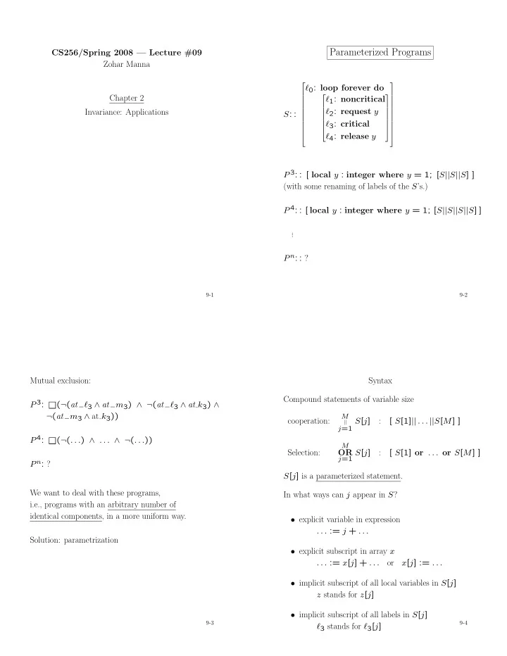
Parameterized Programs

S: :

          

ℓ0: loop forever do

      

ℓ1: noncritical ℓ2: request y ℓ3: critical ℓ4: release y

                 

P 3: : [ local y : integer where y = 1; [S||S||S] ] (with some renaming of labels of the S’s.) P 4: : [ local y : integer where y = 1; [S||S||S||S] ] . . . P n: : ?

9-2

Mutual exclusion: P 3:

0 (¬(at−ℓ3 ∧ at−m3) ∧ ¬(at−ℓ3 ∧ at k3) ∧

¬(at−m3 ∧ at k3)) P 4:

0 (¬(. . .) ∧ . . . ∧ ¬(. . .))

P n: ? We want to deal with these programs, i.e., programs with an arbitrary number of identical components, in a more uniform way. Solution: parametrization

9-3

Syntax Compound statements of variable size cooperation:

M j=1

S[j] : [ S[1]|| . . . ||S[M] ] Selection:

M

OR

j=1 S[j]

: [ S[1] or . . . or S[M] ] S[j] is a parameterized statement. In what ways can j appear in S?

• explicit variable in expression

. . . := j + . . .

• explicit subscript in array x

. . . := x[j] + . . .

• r

x[j] := . . .

• implicit subscript of all local variables in S[j]

z stands for z[j]

• implicit subscript of all labels in S[j]

ℓ3 stands for ℓ3[j]

9-4

SLIDE 2

Example: Program par-sum (Fig. 2.1) (parallel sum of squares) M ≥ 1 z = x[1]2 + x[2]2 + . . . + x[M]2

9-5

Program par-sum-e (Fig. 2.2) (Explicit subscripted parameterized statements

• f par-sum)

We write the short version, but we reason about this one.

9-6

Parameterized transition systems The number M of processes is not fixed, so there is an unbounded number of transitions. To finitely represent these, we use parameterization of transition relations. Example: par-sum The unbounded number of transitions associated with ℓ0 are represented by a single transition relation using parameter j: ρℓ0[j]: move(ℓ0[j], ℓ1[j]) ∧ y′[j] = x[j] ∧ pres({x, z}) where j = 1 . . . M.

9-7

Array Operations Arrays (explicit or implicit) are treated as variables that range over functions: [1 . . . M] → integers Representation of array operations in transition relations:

• Retrieval: y[k]

to retrieve the value of the kth element of array y

• Modification: update(y, k, e)

the resulting array agrees with y on all i, i = k, and y[k] = e

9-8

SLIDE 3

Properties of update update(y, k, e)[k] = e update(y, k, e)[j] = y[j] for j = k Example: par-sum The proper representation of the transition relation for ℓ0[j] is ρ0[j]: move(ℓ0[j], ℓ1[j]) ∧ y′ = update(y, j, x[j]) ∧ pres({x, z})

9-9

Parameterized Programs: Specification Notation:

• Li = {j | ℓi[j] ∈ π}

⊆ {1, . . . , M} The set of indices of processes that currently reside at ℓi

• Ni = |Li|

The number of processes currently residing at ℓi Example: Li = {3, 5} means ℓi[3], ℓi[5] ∈ π and we have Ni = 2 Invariant:

0 (Ni ≥ 0)

Abbreviations: Li1,i2,...,ik = Li1 ∪ Li2 ∪ . . . ∪ Lik Li..j = Li ∪ Li+1 ∪ . . . ∪ Lj Ni1,i2,...,ik = |Li1,i2,...,ik| Ni..j = |Li..j|

9-10

Parameterized Programs: Specification (Con’d) Example: Program mpx-sem (Fig 2.3) M ≥ 2 (multiple mutual exclusion by semaphores) where j ⊕M 1 = (j mod M) + 1 =

• j + 1

if j < M 1 if j = M Elaboration for M = 2: Program mpx-sem-2 (Fig 2.4) mutual exclusion: ∀i, j ∈ [1..M] . i = j . ¬(at−ℓ3[i] ∧ at−ℓ3[j])

• ψ

abbreviated as

0 (N3 ≤ 1)

i.e., the number of processes simultaneously residing at ℓ3 is always less than or equal to 1. Note: ¬(at−ℓ3[i] ∧ at−ℓ3[j]) can be expressed as at−ℓ3[i] + at−ℓ3[j] ≤ 1.

9-11

Program mpx-sem (Fig. 2.3)

9-12

SLIDE 4

Program mpx-sem-2 (Fig. 2.4)

9-13

Parameterized Programs: Verification Objective: prove {ϕ}τ[i]{ϕ} in a uniform way for all i ∈ [1..M] Example: Program mpx-sem (Fig 2.3) M ≥ 2 Prove mutual exclusion:

0 (N3 ≤ 1

• ϕ

) The assertion ϕ is not inductive, therefore we prove the invariance of ϕ1: ∀j . y[j] ≥ 0 ϕ2:

• N3,4 +

M

• j=1

y[j]

• = 1

where N3,4 = Number of processes currently residing at ℓ3 or at ℓ4

9-14

Example: Program mpx-sem (Con’t) Then ϕ can be deducted by monotonicity: ϕ1 ∧ ϕ2 → N3 ≤ 1

• ϕ

since N3 ≤ N3,4 = 1 −

M

• j=1

y[j] ≤ 1 ϕ2 ϕ1

• Proof of

0 (∀j . y[j] ≥ 0

• ϕ1

) B1: . . . ∧ y[1] = 1 ∧ (∀j . 2 ≤ j ≤ M . y[j] = 0)

• Θ

→ ∀j . y[j] ≥ 0

• ϕ1

Note: ∀j . y[j] ≥ 0 stands for ∀j.i ≤ j ≤ M . y[j] ≥ 0

9-15

Example: Program mpx-sem (Con’t) B2: The only transitions that interfere with ϕ1 are τℓ2[i] and τℓ4[i]. ρℓ2[i]: move(ℓ2[i], ℓ3[i]) ∧ y[i] > 0 ∧ y′ = update(y, i, y[i]−1) ρℓ4[i]: move(ℓ4[i], ℓ0[i]) ∧ y′ = update(y, i ⊕M 1, y[i ⊕M 1]+1) ρℓ2[i] implies y[i] > 0 ∧ y′[i] = y[i] − 1 ∧ ∀j . j = i . y′[j] = y[j] ρℓ4[i] implies y′[i ⊕M 1] = y[i ⊕M 1] + 1 ∧ ∀j(j = i ⊕M 1) y′[j] = y[j] We therefore have ∀j . y[j] ≥ 0

• ϕ1

∧

• ρℓ2[i]

ρℓ4[i]

• → ∀j . y′[j] ≥ 0
• ϕ′

1 9-16

SLIDE 5

• Proof of

(N3,4 +

  M

• j=1

y[j]

  = 1)

• ϕ2

B1:

  π = {ℓ0[1], . . . , ℓ0[M]} ∧

y[1] = 1 ∧ (∀j . 2 ≤ j ≤ M . y[j] = 0)

 

• Θ

→ N3,4 +

  M

• j=1

y[j]

  = 1

• ϕ2

B2: Verification conditions: ρℓ2[i] implies: N′

3,4 = N3,4 + 1   M

• j=1

y′[i]

  =   M

• j=1

y[i]

  − 1

9-17

ρℓ4[i] implies: N′

3,4 = N3,4 − 1   M

• j=1

y′[i]

  =   M

• j=1

y[i]

  + 1

Therefore N3,4 +

  M

• j=1

y[i]

  = 1

• ϕ2

∧

• ρℓ2[i]

ρℓ4[i]

• → N′

3,4 +   M

• j=1

y′[i]

  = 1

• ϕ′

2 9-18

Parameterized Programs: Examples Example: readers-writers (Fig 2.11) (readers-writers with generalized semaphores) where request (y, c) = await y ≥ c; y := y − c release (y, c) = y := y + c ∀i, j ∈ [1..M] . i = j . at−ℓ6[i] → ¬(at−ℓ6[j] ∨ at−ℓ3[j])

• ψ
• ϕ1 and ϕ2 are inductive

ϕ1: y ≥ 0 ϕ2: N3,4 + M·N6,7 + y = M

• Therefore

N6,7 > 0 → (N6,7 = 1 ∧ N3,4 = 0) ϕ1, ϕ2 Thus, ψ

9-19

Program read-write(Fig. 2.11)

9-20

SLIDE 6

Example: The Dining Philosophers Problem (multiple resource allocation) Fig 2.14

• M philosophers are seated at a round table
• Each philosopher alternates between a

“thinking” phase and “eating” phase

• M chopsticks, one between every two

philosophers

• A philosopher needs 2 chopsticks

(left & right) to eat

9-21

Dining philosophers setup (Fig. 2.14)

c 2 P 2 c 3 P 3 c 4 P 4 c 5 P 5 c 6 P 6 c 1 P 1

9-22

Program dine (Fig. 2.15) (A simple solution to the dining philosophers problem) Philosopher Pi

• process P[i]

“thinking” phase

• noncritical

“eating” phase

• critical

For philosopher j,

• c[j] represents availability of left chopstick

(c[j] = 1 iff chopstick is available)

• c[j ⊕M 1].............right chopstick

✫✪ ✬✩ ✣✢ ✤✜ ✫✪ ✬✩ ✣✢ ✤✜ ✫✪ ✬✩ ✣✢ ✤✜

Pj−1 c[j] Pj c[j ⊕M 1] Pj⊕M1

9-23

Program dine (Fig. 2.15)

9-24

SLIDE 7

Specification: Chopstick Exclusion ∀j ∈ [1..M] . ¬(at−ℓ4[j] ∧ at−ℓ4[j ⊕M 1])

• ψ

Mutual exclusion between every two adjacent philoso- phers Proof:

• ϕ0 and ϕ1 are inductive

ϕ0: ∀j ∈ [1..M] . c[j] ≥ 0 ϕ1: ∀j ∈ [1..M] . at−ℓ4..6[j] + at−ℓ3..5[j ⊕M 1] + c[j ⊕M 1] = 1

• Then,

at−ℓ4[j] + at−ℓ4[j ⊕M 1] ≤ at−ℓ4··6[j] + at−ℓ3··5[j ⊕M 1] = 1 − c[j ⊕M 1] ≤ 1 ϕ1 ϕ0 Chopstick Exclusion OK

9-25

Problem: possible deadlock (“starvation”) P[1] ℓ2: request c[1]; ℓ3: request c[2] . ↑ . . P[M] ℓ2: request c[M]; ℓ3: request c[1] ↑

✫✪ ✬✩ ✚✙ ✛✘ ✫✪ ✬✩ ✚✙ ✛✘ ✫✪ ✬✩ ✚✙ ✛✘

c[M] PM c[1] P1 c[2] P2

✚ ✙ ✻ ✚ ✙ ✻ ✚ ✙ ✻

9-26

Solution: One Philosopher Excluded (keeping the symmetry)

• Two-room philosophers’ world (Fig 2.18)

Philosophers are “thinking” at the library “eating” at the dining hall When a philosopher finishes “eating” he returns to the library to “think”

• Program dine-excl (Fig 2.17)

Additional semaphore variable r “door keeper” (initally r = M−1) No more than M−1 philosophers are admitted to the dining hall at the same time.

9-27

Two-room philosopher’s world (Fig. 2.18)

Library

c 2 P 2 P 6 c 1 P 1 P 3 c 4 P 4 c 5 P 5 c 6 c 3

9-28

SLIDE 8

Program dine-excl (Fig. 2.17)

9-29

Properties of dine-excl:

• chopstick exclusion

A safety property (in text)

• starvation-free

progress (next book)

• accessibility

ℓ2[j] ⇒

1

ℓ5[j] progress (next book)

9-30

Chapter 3 Precedence

9-31

Proving Precedence Properties

nested waiting-for formulas are of the form p ⇒ qm W (qm−1 · · · (q1 W q0) . . .) also written p ⇒ qm W qm−1 · · · q1 W q0 for assertions p, q0, q1, . . . , qm. Models that satisfy these formulas qm qm−1 q1 interval interval

• • •

interval [ )[ )[ )[ )• p q0 ↑ ↑ p-position q0-position

9-32

SLIDE 9

qi-interval qi qi · · · qi

• May be empty

e.g. p ⇒ q3 W q2 W q1 W q0 q3 q3 q3 q1 q1

• p

q0

• May extend to infinity

q3 q3 q3 q2 q2 q2 · · ·

• p

Note: The following is OK q0

• p

9-33

Simple Precedence: p ⇒ q W r ϕ

• q

q q · · · q

• p

r can be reduced to first-order VCs by verification rule wait: Rule wait (general waiting-for) For assertions p, q, r, ϕ

• W1. p → ϕ ∨ r
• W2. ϕ → q
• W3. {ϕ}T {ϕ ∨ r}

p ⇒ q W r Recall: To show P

q

{ϕ} T {ϕ ∨ r}, we have to show that for every τ ∈ T ρτ ∧ ϕ → ϕ′ ∨ r′ is P-state valid.

9-34

Intermediate Assertion ϕ

• W1. p → ϕ ∨ r

“ϕ weakens p ∧ ¬r” i.e., p ∧ ¬r → ϕ

• W2. ϕ → q

“ϕ strengthens q” q ϕ p ∧ ¬r p r

9-35

Example: Program mux-pet1 (Fig. 3.4) We proved mutual exclusion ψ1: ¬(at−ℓ4 ∧ at−m4) Using invariants χ0: s = 1 ∨ s = 2 χ1: y1 ↔ at−ℓ3..5 χ2: y2 ↔ at−m3..5 χ3: at−ℓ3 ∧ at−m4 → y2 ∧ s = 1 χ4: at−ℓ4 ∧ at−m3 → y1 ∧ s = 2

9-36

SLIDE 10

Example: Program mux-pet1 (Fig. 3.4) (Peterson’s Algorithm for mutual exclusion) local y1, y2: boolean where y1 = f, y2 = f s : integer where s = 1 P1 :: ℓ0 : loop forever do

          

ℓ1 : noncritical ℓ2 : (y1, s) := (t, 1) ℓ3 : await (¬y2) ∨ (s = 1) ℓ4 : critical ℓ5 : y1 := f

          

• P2 ::

m0 : loop forever do

          

m1 : noncritical m2 : (y2, s) := (t, 2) m3 : await (¬y1) ∨ (s = 2) m4 : critical m5 : y2 := f

          

9-37

We want to prove simple precedence ψ2: at−ℓ3 ∧ at−m0..2

• p

⇒ ¬at−m4

• q

W at−ℓ4

r

We try to find an assertion ϕ such that W1 – W3 of rule wait hold Let ϕ : at−ℓ3 ∧ (at−m0..2 ∨ (at−m3 ∧ s = 2))

9-38

W1: at−ℓ3 ∧ at−m0..2

• p

→ at−ℓ3 ∧ (at−m0..2 ∨ · · ·)

• ϕ

∨ · · ·

• r

W2: · · · ∧ (at−m0..2 ∨ (at−m3 ∧ · · ·))

• ϕ

→ ¬at−m4

• q

W3: ρτ ∧ at−ℓ3 ∧ (at−m0..2 ∨ (at−m3 ∧ s = 2))

• ϕ

→ at′

−ℓ3 ∧ (at′ −m0..2 ∨ (at′ −m3 ∧ s′ = 2))

• ϕ′

∨ at′

−ℓ4 r′

Check: ℓ3, m2: OK m3: disabled (with the help of the invariant at−ℓ3..5 ↔ y1, we have y1 = t).

9-39

Proving precedence properties: Systematic derivation of intermediate assertions ϕ [

• )

. p q r Recall: Rule wait (general waiting-for) For assertions p, q, r, ϕ

• W1. p → ϕ ∨ r
• W2. ϕ → q
• W3. {ϕ}T {ϕ ∨ r}

p ⇒ q W r How to find ϕ?

9-40

SLIDE 11

Escape Transition Transition that leads to r-state. q ϕ p r

9-41

Forward propagation Weaken p ∧ ¬r until it becomes an assertion preserved under all nonescape transitions. Based on postcondition: Ψ(V ) = post(τ, ϕ): ∃V 0 . ϕ(V 0) ∧ ρτ(V 0, V ) post(τ, ϕ) characterizes all states that are τ-successors of a ϕ-state. ϕ post(τ, ϕ)

9-42

Example: Postcondition V = {x, y}, ρτ : x′ = x + y ∧ y′ = x, Φ : x = y Then post(τ, Φ) is given by ∃x0, y0 : x0 = y0

• Φ(V 0)

∧ x = x0 + y0 ∧ y = x0

• ρτ(V 0,V )

, which can be simplified to Ψ : x = y + y.

9-43

Forward Propagation: Algorithm Φt - characterizes all states that can be reached from a (p ∧ ¬r)-state without taking an escape transition.

• 1. Φ0 = p ∧ ¬r
• 2. Repeat

Φk+1 = Φk ∨ post(τ, Φk) for any non-escape transition τ Until post(τ, Φt) → Φt [may use invariants] for all non-escape transitions τ If this terminates (it may not), Φt is a good assertion to be used in rule wait. Satisifies W1, W3, but check W2.

9-44

SLIDE 12

Backward propagation Strengthen q until it becomes an assertion preserved under all nonescape transitions. Based on precondition: pre(τ, ϕ): ∀V ′ . ρτ(V, V ′) → ϕ(V ′) pre(τ, ϕ) characterizes all states all of whose τ-successors satisfy ϕ. pre(τ, ϕ) ϕ

9-45

Example: Precondition For Peterson’s Algorithm, consider Γ0 : ¬at m4

• and calculate pre(m3, Γ0):

∀V ′ : at m3 ∧ (¬y1 ∨ s = 2) ∧ at m4′ ∧ · · ·

• ρm3(V,V ′)

→ ¬at m4′

• Γ0(V ′)

. P-equivalent to at m3 → (y1 ∧ s = 2).

9-46

Backward Propagation: Algorithm Γf - characterizes all states that can reach a q-state without taking an escape transition

• 1. Γ0 = q
• 2. Repeat

Γk+1 = Γk ∧ pre(τ, Γk) for any non-escape transition τ Until Γf → pre(τ, Γf) [may use invariants] for all non-escape transitions τ If this terminates (it may not), Γf is a good assertion to be used in rule wait. Satisfies W2, W3, but check W1.

9-47

Backward vs. Forward Γf Φt p ∧ ¬r r q If p ⇒ q W r is P-valid Φt → Γf is P-state valid.

9-48

SLIDE 13

Example: Program mux-pet1 (Fig. 3.4) (Peterson’s Algorithm for mutual exclusion) local y1, y2: boolean where y1 = f, y2 = f s : integer where s = 1 P1 :: ℓ0 : loop forever do

          

ℓ1 : noncritical ℓ2 : (y1, s) := (t, 1) ℓ3 : await (¬y2) ∨ (s = 1) ℓ4 : critical ℓ5 : y1 := f

          

• P2 ::

m0 : loop forever do

          

m1 : noncritical m2 : (y2, s) := (t, 2) m3 : await (¬y1) ∨ (s = 2) m4 : critical m5 : y2 := f

          

9-49

Example: Forward Propagation at ℓ3 ∧ at m0..2

• p

⇒ ¬at m4

• q

W at ℓ4

r

Start with Φ0 : at ℓ3 ∧ at m0..2

• p

. and calculate post(m2, Φ0): ∃ (π0, y0

1, y0 2, s0)

• V 0

: (at ℓ3)0 ∧ (at m0..2)0

• Φ0(V 0)

∧ (at m2)0 ∧ at m3 ∧ ((at ℓ3)0 ↔ at ℓ3) ∧ s = 2 ∧ · · ·

• ρm2(V 0,V )

P-equivalent to Ψ1 : at ℓ3 ∧ at m3 ∧ s = 2, using the invariant ϕ1 : y1 ↔ at ℓ3..5. Thus, Φ1 : at ℓ3 ∧ at m0..2

• Φ0

∨ at ℓ3 ∧ at m3 ∧ s = 2

• Ψ1

,

9-50

Example: Forward Propagation (cont.) i.e., at ℓ3 ∧ (at m0..2 ∨ (at m3 ∧ s = 2)) Φ1 is preserved under all transitions except the escape transition ℓ3, so the process converges.

9-51

Example: Backward Propagation Start with Γ0 : ¬at m4

• q

. We calculated pre(m3, Γ0) above, which is P-equivalent to ∆1 : at m3 → (y1 ∧ s = 2). Thus, Γ1 : ¬at m4

• Γ0

∧ at m3 → (y1 ∧ s = 2)

• ∆1

. Consider transition τm2, and calculate pre(m2, Γ1): ∀V ′ : at m2 ∧ at m3′ ∧ y′

1 = y1 ∧ s′ = 2 ∧ · · ·

• ρm2

→ ¬at m4′ ∧ (at m3′ → (y′

1 ∧ s′ = 2))

• Γ ′

1

. P-equivalent to ∆2 : at m2 → y1.

9-52

SLIDE 14

Example: Backward Propagation (Cont’d) Thus, Γ2 : ¬at m4 ∧ (at m3 → s = 2) ∧ (at m2,3 → y1). Considering transitions τm1, τm0, and τm5 leads to the following sequence: Γ3 : ¬at m4 ∧ (at m3 → s = 2) ∧ (at m1..3 → y1) Γ4 : ¬at m4 ∧ (at m3 → s = 2) ∧ (at m0..3 → y1) Γ5 : ¬at m4 ∧ (at m3 → s = 2) ∧ (at m0..3,5 → y1) By the control invariant at m0..5, Γ5 can be simplified to Γ5 : ¬at m4 ∧ (at m3 → s = 2) ∧ y1.

9-53

Example: Backward Propagation (Cont’d) Calculating pre(ℓ5, Γ5), ∀V ′ : at ℓ5 ∧ y′

1 = f ∧ · · ·

• ρℓ5

→ ¬at m4′ ∧ (at m3′ → s′ = 2) ∧ y′

1

• Γ ′

5

, gives ∆6 : at ℓ5 → f. Propagating Γ5 ∧ ∆6 via τℓ4 gives ∆7 : at ℓ4 → f. Hence, Γ7 : ¬at m4 ∧ (at m3 → s = 2) ∧ at ℓ3, using the invariant ϕ1 : y1 ↔ at ℓ3..5 for simplifica-

• tions. The assertion is preserved under all but the escape

transitions, ending the process.

9-54