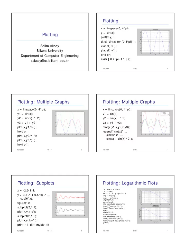
Plotting x = linspace(0, 4* pi); y = sin(x); Plotting - - PDF document

Plotting

Selim Aksoy Bilkent University Department of Computer Engineering saksoy@cs.bilkent.edu.tr

Fall 2004 CS 111 2

Plotting

x = linspace(0, 4* pi); y = sin(x); plot(x,y); title( 'sin(x) for [0,4\pi]' ); xlabel( 'x' ); ylabel( 'y' ); grid on; axis( [ 0 4* pi -1 1 ] );

Fall 2004 CS 111 3

Plotting: Multiple Graphs

x = linspace(0, 4* pi); y1 = sin(x); y2 = sin(x) .^ 2; y3 = y1 + y2; plot(x,y1,'b-'); hold on; plot(x,y2,'r--'); plot(x,y3,'g:'); hold off;

Fall 2004 CS 111 4

Plotting: Multiple Graphs

x = linspace(0, 4* pi); y1 = sin(x); y2 = sin(x) .^ 2; y3 = y1 + y2; plot(x,y1,x,y2,x,y3); legend( 'sin(x)', ... 'sin(x)^ 2', ... 'sin(x) + sin(x)^ 2' );

Fall 2004 CS 111 5

Plotting: Subplots

x = -2:0.1:4; y = 3.5 .^ (-0.5* x) .* ... cos(6* x); figure(1); subplot(2,1,1); plot(x,y,'r-o'); subplot(2,1,2); plot(x,y,'k--* '); print -f1 -dtiff myplot.tif

Fall 2004 CS 111 6

Plotting: Logarithmic Plots

r = 16000; c = 1.0e-6; f = 1:2:1000; res = 1 ./ ( 1 + j* 2* pi* f* r* c ); amp = abs(res); phase = angle(res); subplot (2,1,1); loglog(f,amp); title( 'Amplitude response' ); xlabel( 'Frequency (Hz)' ); ylabel( 'Output/Input ratio' ); grid on; subplot (2,1,2); semilogx(f,phase); title( 'Phase response' ); xlabel( 'Frequency (Hz)' ); ylabel( 'Output -Input phase (rad)' ); grid on;

Fall 2004 CS 111 7

Plotting Summary

plot(x,y)

linear plot of vector y vs. vector x

title('text'), xlabel('text'), ylabel('text')

labels the figure, x-axis and y-axis

grid on/off

adds/removes grid lines

hold on/off

allows/disallows adding subsequent graphs to the current graph

Fall 2004 CS 111 8

Plotting Summary

legend( 'string1', 'string2', 'string3', ... )

adds a legend using the specified strings

v = axis

returns a row vector containing the scaling for the current plot

axis( [ xmin xmax ymin ymax ] )

sets axes’ limits

Fall 2004 CS 111 9

Plotting Summary

• :
• .
• .
• x

+ * s d v ^ < > p h b g r c m y k solid dotted dashdot dashed point circle x-mark plus star square diamond triangle (down) triangle (up) triangle (left) triangle (right) pentagram hexagram blue green red cyan magenta yellow black line style line marker line color

Fall 2004 CS 111 10

Plotting Summary

semilogy(x,y), semilogx(x,y), loglog(x,y)

logarithmic plots of vector y vs. vector x

figure(k)

makes figure k the current figure

subplot(m,n,p)

breaks the figure window into an m-by-n matrix of small axes and selects the pth axes for the current plot

clf

clears current figure

Fall 2004 CS 111 11

Plotting Summary

print –f< handle> -d< device> < filename>

saves the figure with the given handle in the format specified by the device

• deps

Encapsulated PostScript

• depsc

Encapsulated Color PostScript

• deps2

Encapsulated Level 2 PostScript

• depsc2

Encapsulated Level 2 Color PostScript

• djpeg<nn>

JPEG image with quality level of nn

• dtiff

TIFF image

• dpng

Portable Network Graphics image

Fall 2004 CS 111 12

Plotting Examples

Line plot

x = -2:0.01:4; y = 3.5.^ (-0.5* x).* cos(6* x); plot(x,y); line([0 0],[-3 3],'color','r');

Pie plot

grades = [ 11 18 26 9 5 ]; pie(grades);

Fall 2004 CS 111 13

Plotting Examples

Vertical bar plot

y = 1988:1994; s = [ 8 12 20 22 18 24 27 ]; bar(y,s,'r');

Horizontal bar plot

y = 1988:1994; s = [ 8 12 20 22 18 24 27 ]; barh(y,s,'g');

Fall 2004 CS 111 14

Plotting Examples

Stairs plot

y = 1988:1994; s = [ 8 12 20 22 18 24 27 ]; stairs(y,s);

Stem plot

y = 1988:1994; s = [ 8 12 20 22 18 24 27 ]; stem(y,s);

Fall 2004 CS 111 15

Plotting Examples

Histogram

x = randn(1,100); hist(x,10); hist(x,20);

Fall 2004 CS 111 16

Plotting Examples

Polar plot

t = linspace(0,2* pi,200); r = 3 * cos(0.5* t).^ 2 + t; polar(t,r);

Compass plot

u = [ 3 4 -2 -3 0.5 ]; v = [ 3 1 3 -2 -3 ] ; compass(u,v);

Fall 2004 CS 111 17

Plotting Examples

Error bar plot

x = 1:10; y = sin(x); e = std(y) * ones(size(x)); errorbar(x,y,e);