Precision determination of the top-quark mass Sven-Olaf Moch - - PowerPoint PPT Presentation

precision determination of the top quark mass
SMART_READER_LITE
LIVE PREVIEW

Precision determination of the top-quark mass Sven-Olaf Moch - - PowerPoint PPT Presentation

Precision determination of the top-quark mass Sven-Olaf Moch Universit at Hamburg Theoretical Physics Seminar , Liverpool, Mar 04,


slide-1
SLIDE 1

Precision determination of the top-quark mass

Sven-Olaf Moch

Universit¨ at Hamburg ————————————————————————————————————–

Theoretical Physics Seminar, Liverpool, Mar 04, 2015

Sven-Olaf Moch Precision determination of the top-quark mass – p.1

slide-2
SLIDE 2

Introduction (I)

Classical mechanics

  • Mass is defined as product of density and volume of matter
  • classical concept

Sven-Olaf Moch Precision determination of the top-quark mass – p.2

slide-3
SLIDE 3

Introduction (I)

Classical mechanics

  • Mass is defined as product of density and volume of matter
  • classical concept
  • The quantity of matter is that which arises

jointly from its density and magnitude. A body twice as dense in double the space is quadruple in quantity. This quantity I designate by the name of body or of mass.

Newton

Sven-Olaf Moch Precision determination of the top-quark mass – p.2

slide-4
SLIDE 4

Introduction (I)

Classical mechanics

  • Mass is defined as product of density and volume of matter
  • classical concept
  • The quantity of matter is that which arises

jointly from its density and magnitude. A body twice as dense in double the space is quadruple in quantity. This quantity I designate by the name of body or of mass.

Newton

Atomic theory

  • Mass is conserved Lavoisier
  • Mass of body is sum of mass
  • f its constituents

M(X) = NAma(X) Avogadro

Sven-Olaf Moch Precision determination of the top-quark mass – p.2

slide-5
SLIDE 5

Introduction (II)

Kilogram

The kilogram is the unit of mass; it is equal to the mass of the international prototype of the kilogram.

  • International prototype kilogram (IPK):

made in 1889, 39 mm high, alloy of platinum and iridium

Orginal des Bureau International des Poids et Mesures

Sven-Olaf Moch Precision determination of the top-quark mass – p.3

slide-6
SLIDE 6

Introduction (II)

Kilogram

The kilogram is the unit of mass; it is equal to the mass of the international prototype of the kilogram.

  • International prototype kilogram (IPK):

made in 1889, 39 mm high, alloy of platinum and iridium

Orginal des Bureau International des Poids et Mesures

Special relativity

  • Equivalence principle

E = mc2 Einstein

Sven-Olaf Moch Precision determination of the top-quark mass – p.3

slide-7
SLIDE 7

Introduction (II)

Kilogram

The kilogram is the unit of mass; it is equal to the mass of the international prototype of the kilogram.

  • International prototype kilogram (IPK):

made in 1889, 39 mm high, alloy of platinum and iridium

Orginal des Bureau International des Poids et Mesures

Special relativity

  • Equivalence principle

E = mc2 Einstein

Standard Model

  • Higgs boson gives mass to matter fields via Higgs-Yukawa coupling
  • large top-quark mass mt

Sven-Olaf Moch Precision determination of the top-quark mass – p.3

slide-8
SLIDE 8

Quantum field theory

QCD

  • Classical part of QCD Lagrangian

L = −1 4 F a

µνF µν b

+

  • flavors

¯ qi (i / D − mq)ij qj

  • field strength tensor F a

µν and matter fields qi, ¯

qj

  • covariant derivative Dµ,ij = ∂µδij + igs (ta)ij Aa

µ

  • Formal parameters of the theory (no observables)
  • strong coupling αs = g2

s/(4π)

  • quark masses mq
  • Parameters of Lagrangian have no unique physical interpretation
  • radiative corrections require definition of renormalization scheme

Challenge

  • Suitable observables for measurements of αs, mq, . . .
  • comparison of theory predictions and experimental data

Sven-Olaf Moch Precision determination of the top-quark mass – p.4

slide-9
SLIDE 9

Coupling constant renormalization

  • Running coupling constant αs from radiative corrections, e.g. one loop

– screening (like in QED) – anti-screening (color charge ofg)

  • QCD beta function µ2 d

dµ2 αs(µ) = β(αs)

  • perturbative expansion

to four loops

van Ritbergen, Vermaseren, Larin ‘97

  • very good convergence
  • f perturbative series

even at low scales

1.0 1.5 2.0 2.5 3.0 0.25 0.30 0.35 0.40

running coupling

µ αs(µ)

Sven-Olaf Moch Precision determination of the top-quark mass – p.5

slide-10
SLIDE 10

Quark mass renormalization

  • Heavy-quark self-energy Σ(p, mq)

Σ Σ + Σ + + . . .

= i / p − mq − Σ(p, mq)

QCD

  • QCD corrections to self-energy Σ(p, mq)

t g

  • dimensional regularization D = 4 − 2ǫ
  • one-loop: UV divergence 1/ǫ (Laurent expansion)

Σ(1),bare(p, mq) = αs 4π µ2 m2

q

ǫ (/ p − mq)

  • −CF 1

ǫ + fin.

  • + mq
  • 3CF 1

ǫ + fin.

  • Relate bare and renormalized mass parameter mbare

q

= mren

q

+ δmq

= + + + . . . Σren(p, mq) (Zψ − 1)/ p − (Zm − 1)mq

Sven-Olaf Moch Precision determination of the top-quark mass – p.6

slide-11
SLIDE 11

Quark mass renormalization

  • Heavy-quark self-energy Σ(p, mq)

Σ Σ + Σ + + . . .

= i / p − mq − Σ(p, mq)

EW sector

  • EW corrections to top-quark self-energy
  • on-shell intermediate (virtual) W-boson
  • mt complex parameter with imaginary part Γt = 2.0 ± 0.7 GeV
  • Γt > 1 GeV: top-quark decays before it hadronizes

t W t b

Sven-Olaf Moch Precision determination of the top-quark mass – p.6

slide-12
SLIDE 12

Mass renormalization scheme

Pole mass

  • Based on (unphysical) concept of top-quark being a free parton
  • mren

q

coincides with pole of propagator at each order / p − mq − Σ(p, mq)

  • /

p=mq

→ / p − mpole

q

  • Definition of pole mass ambiguous up to corrections O(ΛQCD)
  • heavy-quark self-energy Σ(p, mq) receives contributions from regions
  • f all loop momenta – also from momenta of O(ΛQCD)
  • bound from lattice QCD: ∆mq ≥ 0.7 · ΛQCD ≃ 200 MeV

Bauer, Bali, Pineda ’11

MS scheme

  • MS mass definition
  • one-loop minimal subtraction

δm(1)

q

= mq αs 4π 3CF 1 ǫ − γE + ln 4π

  • MS scheme induces scale dependence: m(µ)

Sven-Olaf Moch Precision determination of the top-quark mass – p.7

slide-13
SLIDE 13

Running quark mass

Scale dependence

  • Renormalization group equation for scale dependence
  • mass anomalous dimension γ known to four loops

Chetyrkin ‘97; Larin, van Ritbergen, Vermaseren ‘97

  • µ2 ∂

∂µ2 + β(αs) ∂ ∂αs

  • m(µ) = γ(αs)m(µ)
  • Plot mass ratio mt(163GeV)/mt(µ)

90 100 110 120 130 140 150 160 0.96 0.97 0.98 0.99 1.00

running top quark mass

µ m(µ)

Sven-Olaf Moch Precision determination of the top-quark mass – p.8

slide-14
SLIDE 14

Scheme transformations

  • Conversion between different renormalization schemes possible in

perturbation theory

  • Relation for pole mass and MS mass
  • known to four loops in QCD Gray, Broadhurst, Gräfe, Schilcher ‘90;

Chetyrkin, Steinhauser ‘99; Melnikov, v. Ritbergen ‘99; Marquard, Smirnov, Smirnov, Steinhauser ‘15

  • EW sector known to O(αEWαs)

Jegerlehner, Kalmykov ‘04; Eiras, Steinhauser ‘06

  • example: one-loop QCD

mpole = m(µ)

  • 1 + αs(µ)

4π 4 3 + ln

  • µ2

m(µ)2

  • + . . .
  • Sven-Olaf Moch

Precision determination of the top-quark mass – p.9

slide-15
SLIDE 15

Top-quark mass

What is the value of the top-quark mass ?

mt = ?

Sven-Olaf Moch Precision determination of the top-quark mass – p.10

slide-16
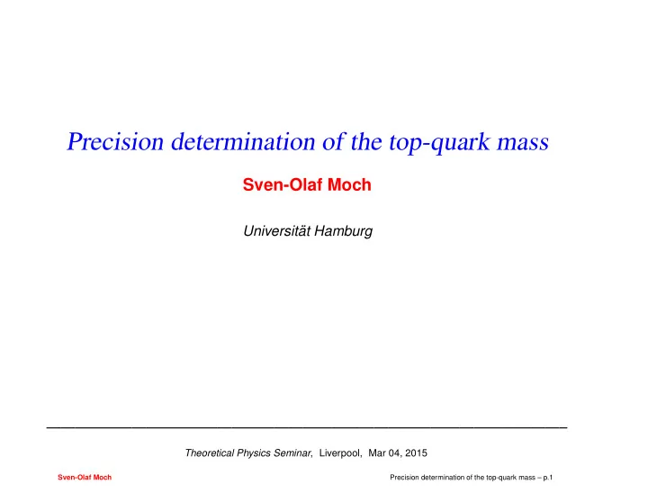
SLIDE 16

Some Answers

[GeV]

top

m 165 170 175 180 185 1 17

LHC September 2013 0.88) ± 0.26 ± (0.23

0.95 ± 173.29

Tevatron March 2013 (Run I+II) 0.61) ± 0.36 ± (0.51

0.87 ± 173.20

prob.=93%

2

χ / ndf =4.3/10

2

χ

World comb. 2014 0.67) ± 0.24 ± (0.27

0.76 ± 173.34

  • 1

= 3.5 fb

int

L

CMS 2011, all jets 1.23) ± (0.69

1.41 ± 173.49

  • 1

= 4.9 fb

int

L

CMS 2011, di-lepton 1.46) ± (0.43

1.52 ± 172.50

  • 1

= 4.9 fb

int

L

CMS 2011, l+jets 0.97) ± 0.33 ± (0.27

1.06 ± 173.49

  • 1

= 4.7 fb

int

L

ATLAS 2011, di-lepton 1.50) ± (0.64

1.63 ± 173.09

  • 1

= 4.7 fb

int

L

ATLAS 2011, l+jets 1.35) ± 0.72 ± (0.23

1.55 ± 172.31

  • 1

= 5.3 fb

int

L

D0 RunII, di-lepton 1.38) ± 0.55 ± (2.36

2.79 ± 174.00

  • 1

= 3.6 fb

int

L

D0 RunII, l+jets 1.16) ± 0.47 ± (0.83

1.50 ± 174.94

  • 1

= 8.7 fb

int

L

+jets

miss T

CDF RunII, E 0.86) ± 1.05 ± (1.26

1.85 ± 173.93

  • 1

= 5.8 fb

int

L

CDF RunII, all jets 1.04) ± 0.95 ± (1.43

2.01 ± 172.47

  • 1

= 5.6 fb

int

L

CDF RunII, di-lepton 3.13) ± (1.95

3.69 ± 170.28

  • 1

= 8.7 fb

int

L

CDF RunII, l+jets 0.86) ± 0.49 ± (0.52

1.12 ± 172.85

  • 1
  • 8.7 fb
  • 1

= 3.5 fb

int

combination - March 2014, L

top

Tevatron+LHC m ATLAS + CDF + CMS + D0 Preliminary

) syst. iJES stat. total ( Previous Comb. Sven-Olaf Moch Precision determination of the top-quark mass – p.11

slide-17
SLIDE 17

World combination

Experiment: ATLAS, CDF, CMS & D0 coll. 1403.4427

mt = 173.34 ± 0.76 GeV

Sven-Olaf Moch Precision determination of the top-quark mass – p.12

slide-18
SLIDE 18

World combination

Experiment: ATLAS, CDF, CMS & D0 coll. 1403.4427

mt = 173.34 ± 0.76 GeV

In all measurements considered in the present combination, the analyses are calibrated to the Monte Carlo (MC) top-quark mass definition.

Sven-Olaf Moch Precision determination of the top-quark mass – p.12

slide-19
SLIDE 19

World combination

Experiment: ATLAS, CDF, CMS & D0 coll. 1403.4427

mt = 173.34 ± 0.76 GeV

In all measurements considered in the present combination, the analyses are calibrated to the Monte Carlo (MC) top-quark mass definition.

Theory:

That is, we can state as the final result for the likely relation between the top-quark mass measured using a given Monte Carlo event generator ("MC") and the pole mass as mpole = mMC + Q0 [αs(Q0)c1 + . . . ] where Q0 ∼ 1 GeV and c1 is unknown, but presumed to be of order 1 and, according to the argument above, presumed to be positive.

  • A. Buckley et al. arXiv:1101.2599

Sven-Olaf Moch Precision determination of the top-quark mass – p.12

slide-20
SLIDE 20

Rates, shapes and peaks

  • Rates and shapes of distributions offer possibility for top mass

determination with well-defined renormalization scheme

  • Requirements:
  • theory predictions at least to NLO in QCD
  • sufficiently large sensitivity S to mt (kinematics)
  • ∆σt¯

t

σt¯

t

  • ≃ S ×
  • ∆mt

mt

  • Observables (examples):
  • inclusive cross section
  • distributions for t¯

t + 1jet samples

  • kinematic reconstruction of top mass (Monte Carlo mass)

Sven-Olaf Moch Precision determination of the top-quark mass – p.13

slide-21
SLIDE 21

Top mass from total cross section

µ µ p fi i p j fj Q X

  • QCD factorization

σpp→X =

  • ij

fi(µ2) ⊗ fj(µ2) ⊗ ˆ σij→X

  • αs(µ2), Q2, µ2, m2

X

  • Joint dependence on non-perturbative parameters:

parton distribution functions fi, strong coupling αs, masses mX

  • Intrinsic limitation in total cross section through sensitivity S ≃ 5
  • ∆σt¯

t

σt¯

t

  • ≃ 5 ×
  • ∆mt

mt

  • Sven-Olaf Moch

Precision determination of the top-quark mass – p.14

slide-22
SLIDE 22

Total cross section

Exact result at NNLO in QCD

Czakon, Fiedler, Mitov ‘13

σpp → tt [pb] at LHC8

  • NNLO

NLO LO mt

pole

[GeV] 100 200 300 400 500 600 150 160 170 180 190 σpp → tt [pb] at LHC8

  • mt

pole

= 173 GeV µ/mt

pole

100 120 140 160 180 200 220 240 260 1

  • NNLO perturbative corrections (e.g. at LHC8)
  • K-factor (NLO → NNLO) of O(10%)
  • scale stability at NNLO of O(±5%)

Sven-Olaf Moch Precision determination of the top-quark mass – p.15

slide-23
SLIDE 23

Total cross section with running mass

Comparison pole mass vs. MS mass (I)

Dowling, S.M. ‘13

σpp → tt [pb] at LHC8

  • NNLO

NLO LO mt

pole

[GeV] 100 200 300 400 500 600 150 160 170 180 190 σpp → tt [pb] at LHC8

  • NNLO

NLO LO m(m) [GeV] 100 200 300 400 500 600 140 150 160 170 180

pole mass

MS mass

  • NNLO cross section with running mass significantly improved
  • good apparent convergence of perturbative expansion
  • small theoretical uncertainity form scale variation

Sven-Olaf Moch Precision determination of the top-quark mass – p.16

slide-24
SLIDE 24

Total cross section with running mass

Comparison pole mass vs. MS mass (II)

Dowling, S.M. ‘13

σpp → tt [pb] at LHC8

  • mt

pole

= 173 GeV µ/mt

pole

100 120 140 160 180 200 220 240 260 1 σpp → tt [pb] at LHC8

  • m(m) = 163 GeV

µ/m(m) 100 120 140 160 180 200 220 240 260 1

pole mass

MS mass

  • NNLO cross section with running mass significantly improved
  • good apparent convergence of perturbative expansion
  • small theoretical uncertainity form scale variation

Sven-Olaf Moch Precision determination of the top-quark mass – p.16

slide-25
SLIDE 25

Top cross section data in ABM12 fit

  • Fit with correlations
  • g(x) and αs(MZ) already well constrained by global fit (no changes)
  • for fit with χ2/NDP = 5/5 obtain value of mt(mt) = 162.3 ± 2.3 GeV

(equivalent to pole mass mt = 171.2 ± 2.4 GeV) Alekhin, Blümlein, S.M. ‘13

  • χ2-profile steeper for pole mass (bigger impact of top-quark data and

greater sensitivity to theoretical uncertainty at NNLO)

mt(mt)/GeV χ2 running mass mt(pole)/GeV pole mass mt(mt)/GeV χ

2 t

NDP=5 running mass mt(pole)/GeV pole mass

Sven-Olaf Moch Precision determination of the top-quark mass – p.17

slide-26
SLIDE 26

Top-quark pairs with one jet

  • LHC: large rates for production of t¯

t-pairs with additional jets

  • NLO QCD corrections for t¯

t + 1jet Dittmaier, Uwer, Weinzierl ‘07-‘08

  • scale dependence greatly reduced at NLO
  • corrections for total rate at scale µr = µf = mt are almost zero

g g t g

  • t

g g t

  • t

g g g t g

  • t

g g t g

  • t

q

  • q

t

  • t

g q

  • q

t g

  • t

q

  • q

t g

  • t

LO (CTEQ6L1) NLO (CTEQ6M)

pT,jet > 20GeV √s = 14 TeV pp → t¯ t+jet+X µ/mt σ[pb]

10 1 0.1 1500 1000 500

  • Additional jet raises kinematical threshold
  • invariant mass √st¯

t+1jet

Sven-Olaf Moch Precision determination of the top-quark mass – p.18

slide-27
SLIDE 27

Top mass with t¯

t + jet-samples

  • Normalized-differential t¯

t + jet cross section

Alioli, Fernandez, Fuster, Irles, S.M., Uwer, Vos ‘13

R(mt, ρs) = 1 σt¯

t+1jet

dσt¯

t+1jet

dρs (mt, ρs)

  • variable ρs =

2·m0 √st¯

t+1jet with invariant mass of t¯

t + 1jet system and fixed scale m0 = 170 GeV

  • Significant mass dependence for 0.4 ≤ ρs ≤ 0.5 and 0.7 ≤ ρs

)

s

ρ ,

pole t

(m

R

0.5 1 1.5 2 2.5 3 3.5

160 GeV, CTEQ6.6 170 GeV, CTEQ6.6 170 GeV, MSTW 180 GeV, CTEQ6.6

s

ρ

0.2 0.3 0.4 0.5 0.6 0.7 0.8

ratio

1 2 3

Sven-Olaf Moch Precision determination of the top-quark mass – p.19

slide-28
SLIDE 28

Mass sensitivity of t¯

t + jet-samples

  • Differential cross section R(mt, ρs)
  • good pertubative stability, small theory uncertainties, small

dependence on experimental uncertainties, . . .

  • Increased sensitivity for system t¯

t + jet compared

  • ∆R

R

  • ≃ (mtS) ×
  • ∆mt

mt

  • ρ

0.2 0.3 0.4 0.5 0.6 0.7 0.8 0.9

]

  • 1

[GeV

)

ρ

( S

0.05 0.1 0.15

)

ρ

( S

×

t pole

m

25.5 17 8.5 +1Jet t t = 10 GeV

pole t

m ∆ = 5 GeV

pole t

m ∆ t t = 10 GeV

pole t

m ∆ = 5 GeV

pole t

m ∆

  • ATLAS analysis ongoing (preliminary mass reported at Top2014)

Sven-Olaf Moch Precision determination of the top-quark mass – p.20

slide-29
SLIDE 29

Monte Carlo mass

  • Hard interaction and parton emission in QCD followed by hadronization
  • Top-quark decays on shell (e.g. leptonic decay t → bW → bl¯

νl)

[picture by B.Webber]

  • Intuition: Monte Carlo mass identified with pole mass due to kinematics

m2

q = E2 q − p2

  • Caveat: heavy quarks in QCD interact with potential due to gluon field

Sven-Olaf Moch Precision determination of the top-quark mass – p.21

slide-30
SLIDE 30

Kinematic reconstruction

  • Current methods based on reconstructed physics objects
  • jets, identified charged leptons,

missing transverse energy

  • m2

t = (pW −boson + pb−jet)2

l ¯ νl t W b

Template method

  • Distributions of kinematically reconstructed top mass values compared to

templates for nominal top mass values

  • distributions rely on parton shower predictions
  • uncertainties from variation of Monte Carlo parameters

Sven-Olaf Moch Precision determination of the top-quark mass – p.22

slide-31
SLIDE 31

Hard scattering process

  • Born process (q¯

q-channel) with leptonic decay t → bl¯ νl

¯ q q ¯ t b l ¯ νl W t g

Sven-Olaf Moch Precision determination of the top-quark mass – p.23

slide-32
SLIDE 32

Radiative corrections

  • Virtual corrections (examples): gluon exchange
  • box diagram (left) and vertex corrections (right)
  • infrared divergences cancel against real emission contributions

¯ q q ¯ t b l ¯ νl W t g g ¯ q q ¯ t b l ¯ νl W t g g

  • Mass renormalization from

self-energy corrections to top-quark

¯ q q ¯ t b l ¯ νl W t g g

Sven-Olaf Moch Precision determination of the top-quark mass – p.24

slide-33
SLIDE 33

Radiative corrections

  • Real corrections (examples): gluon emission
  • phase space integration → infrared divergences (soft/collinear

singularities)

¯ q q ¯ t b l ¯ νl W t g g ¯ q q ¯ t b l ¯ νl W t g g

  • Parton shower MC
  • emission probability modeled by Sudakov exponential with cut-off Q0
  • leading logarithmic accuracy

  • Q2, Q2
  • = exp
  • −CF αs

2π ln Q2 Q2

  • subtraction of IR contributions at hadronization scale Q0 ≃ O(1)GeV

Sven-Olaf Moch Precision determination of the top-quark mass – p.24

slide-34
SLIDE 34

Mass of heavy-quark jet (I)

  • Cross section for invariant mass of jet Mt(¯

t) in e+e− → t¯

t

  • Back-to-back heavy-quark jets with collinear parton emission define

hemispheres Fleming, Hoang, Mantry, Stewart ‘07

thrust axis soft particles

n-collinear n-collinear

hemisphere-a hemisphere-b

  • Cross section factorization in effective theory (SCET)

d2σ dM 2

t dM 2 ¯ t

= σ0 H(Q, m, µ)

  • hard fct.
  • dℓ+dℓ− B+(Mt, Γt, µ)
  • jet fct.

B−(M¯

t, Γt, µ)

  • jet fct.

S(ℓ+, ℓ−, µ)

  • soft fct.
  • hierarchy of scales Q ≫ mt ≫ Γt ≫ ΛQCD and |Mt − mt| ≃ Γt

Sven-Olaf Moch Precision determination of the top-quark mass – p.25

slide-35
SLIDE 35

Mass of heavy-quark jet (II)

  • Computation of heavy-quark jet function from discontinuity of

heavy-quark propagator connected by light-like Wilson lines Wn(0)W †

n(x)

B+(v+ · k, Γt) = −1 8πNcmDisc

  • d4x eik·x0|T{¯

hv+(0)Wn(0)W †

n(x)hv+(x)}|0

  • Computation of B± in perturbation theory with well-defined mass scheme
  • Breit-Wigner resonance at tree level

B±(ˆ s, Γt) = 1 4πmDisc.

  • i

v± · k + iΓt/2

  • =

1 πm Γt ˆ s2 + Γ2

t

  • Stable peak position at higher orders

Hoang, Stewart ‘08

  • Mass renormalization with

short-distance mass mpole = mshort distance + δm

  • short-distance mass mMSR(R)

probes scale of hard interaction: R ≃ Γt

jet-mass scheme

LL tree NLL NNLL

B m

M

t (GeV)

171 172 173 174 175 0.10 0.20 0.25 0.15 0.05 0.00

Sven-Olaf Moch Precision determination of the top-quark mass – p.26

slide-36
SLIDE 36

Conversion Monte Carlo mass to pole mass (I)

Assumption

  • Identify Monte Carlo mass mMC with short distance mass mMSR(R) at

low scale O(1) GeV

  • choice for range of scale R ≃ 1 . . . 9GeV

mMC = mMSR(R = 3+6

−2GeV)

Sven-Olaf Moch Precision determination of the top-quark mass – p.27

slide-37
SLIDE 37

Conversion Monte Carlo mass to pole mass (II)

Strategy

  • Use perturbation theory

to convert mMSR(R) to mpole

  • Running of mMSR(R) mass

Hoang, Stewart ‘08

✵ ✶ ✵
✶ ✵✵ ❘ ✶ ✵ ✶ ✁ ✵ ✶ ✂ ✵ ✶✄ ✵ ♠☎ ✆ ✝ ✆ ✞ ♠☎ ✆ ✝ ✟ ❚ ❡ ✠✡ ☛ ☞ ✌✍ ♠☎ ♠✝
  • Choice 1: run mMSR(R) from low scale to R = mt: mMSR(R) → m(m)

and convert from m(m) to pole mass

[arXiv:1405.4781]

mMSR(1) mMSR(3) mMSR(9) m(m) mpl

1lp

mpl

2lp

mpl

3lp

173.72 173.40 172.78 163.76 171.33 172.95 173.45

  • Choice 2: convert from mMSR(R) at low scale directly to pole mass

mMSR(1) mMSR(3) mMSR(9) mpl

1lp

mpl

2lp

mpl

3lp

173.72 173.40 172.78 173.72 173.87 173.98

Sven-Olaf Moch Precision determination of the top-quark mass – p.28

slide-38
SLIDE 38

Conversion Monte Carlo mass to pole mass (III)

Summary

mpole = 173.34 ± 0.76 GeV (exp) + ∆m(th) with ∆m(th) =

+0.32 −0.62 GeV (mMC → mMSR(3GeV)) + 0.50 GeV (m(m) → mpole)

and combined ∆m(th) =

+0.82 −0.62GeV

In addition, unknown systematic mass shift O(1) GeV due to non-perturbative effects on peak position of invariant jet-mass distribution M peak with decaying top-quark for short distance mass mt M peak = mt + Γt(αs + α2

s + . . .) + QΛQCD

mt

Sven-Olaf Moch Precision determination of the top-quark mass – p.29

slide-39
SLIDE 39

Non-perturbative corrections

  • Simulation of top mass measurement Skands, Wicke ’07
  • test of different Monte Carlo tunes for non-perturbative physics /

colour reconnection

  • calibration offsets before/after scaling with jet energy scale

corrections

  • Parton shower models:
  • pT -ordered (blue);
  • virtuality ordered (green)
  • Uncertainty in parton shower

models (non-perturbative) is O(±500) MeV

∆mfit

top

∆mscaled

top

  • ∆mt
  • 10
  • 5

5

Tune A Tune A-CR Tune A-PT Tune DW Tune BW S0 S1 S2 NoCR

Sven-Olaf Moch Precision determination of the top-quark mass – p.30

slide-40
SLIDE 40

Higgs boson mass

Experimental result

Atlas arXiv:1307.1427; CMS coll. arXiv:1312.5353; (average arXiv:1303.3570)

mH = 125.15 ± 0.24GeV

Sven-Olaf Moch Precision determination of the top-quark mass – p.31

slide-41
SLIDE 41

Higgs potential

Renormalization group equation

  • Quantum corrections to Higgs potential V (Φ) = λ
  • Φ†Φ − v

2

  • 2
  • Radiative corrections to Higgs self-coupling λ
  • electro-weak couplings g and g′ of SU(2) and U(1)
  • top-Yukawa coupling yt

16π2 dλ dQ = 24λ2 −

  • 3g′2 + 9g2 − 12y2

t

  • λ + 3

8g′4 + 3 4g′2g2 + 9 8g4 − 6y4

t + . . .

H H H H H H H H H H H H H H H H

H H H H t H H H H V H H H H

Sven-Olaf Moch Precision determination of the top-quark mass – p.32

slide-42
SLIDE 42

Higgs potential

Triviality

  • Large mass implies large λ
  • renormalization group equation dominated by first term

16π2 dλ dQ ≃ 24λ2 − → λ(Q) = m2

H

2v2 −

3 2π2 m2 H ln(Q/v)

  • λ(Q) increases with Q
  • Landau pole implies cut-off Λ
  • scale of new physics smaller than Λ to restore stability
  • upper bound on mH for fixed Λ

Λ ≤ v exp 4π2v2 3m2

H

  • Triviality for Λ → ∞
  • vanishing self-coupling λ → 0 (no interaction)

Sven-Olaf Moch Precision determination of the top-quark mass – p.32

slide-43
SLIDE 43

Higgs potential

Vacuum stability

  • Small mass
  • renormalization group equation dominated by yt

16π2 dλ dQ ≃ −6y4

t

− → λ(Q) = λ0 −

3 8π2 y4 0 ln(Q/Q0)

1 −

9 16π2 y2 0 ln(Q/Q0)

  • λ(Q) decreases with Q
  • Higgs potential unbounded from below for λ < 0
  • λ = 0 for λ0 ≃

3 8π2 y4 0 ln(Q/Q0)

  • Vacuum stability

Λ ≤ v exp 4π2m2

H

3y4

t v2

  • scale of new physics smaller than Λ to ensure vacuum stability
  • lower bound on mH for fixed Λ

Sven-Olaf Moch Precision determination of the top-quark mass – p.32

slide-44
SLIDE 44

Implications on electroweak vacuum

  • Relation between Higgs mass mH and top-quark mass mt
  • condition of absolute stability of electroweak vacuum λ(µ) ≥ 0
  • extrapolation of Standard Model up to Planck scale MP
  • λ(MP ) ≥ 0 implies lower bound on Higgs mass mH

mH ≥ 129.6 + 2.0×

  • mpole

t

− 173.34 GeV

  • − 0.5×

αs(MZ) − 0.1184 0.0007

  • ± 0.3 GeV
  • recent NNLO analyses Bezrukov, Kalmykov, Kniehl, Shaposhnikov ‘12;

Degrassi, Di Vita, Elias-Miro, Espinosa, Giudice et al. ‘12; Buttazzo, Degrassi, Giardino, Giudice, Sala, Salvio, Strumia ‘13

  • uncertainity in results due to αs and mt (pole mass scheme)
  • Top-quark mass from total cross section (well-defined scheme)
  • mMS

t

(mt) = 162.3 ± 2.3 ± 0.7 GeV implies in pole mass scheme mpole

t

= 171.2 ± 2.4 ± 0.7 GeV

  • mass determination accounts for correlation with gluon PDF and

αS(MZ)

Sven-Olaf Moch Precision determination of the top-quark mass – p.33

slide-45
SLIDE 45

Fate of the universe

✵ ✺ ✵ ✶ ✵✵ ✶✺ ✵ ✷ ✵✵ ✵ ✺ ✵ ✶ ✵✵ ✶✺ ✵ ✷ ✵✵ ❍✁✁✂ ♠✄ ✂✂ ▼ ❤ ✐
✆ ❚ ✝ ✞ ✟ ✠ ✡ ✡ ☛ t ☞ ✌ ✍ ✎ ✏ ■ ✐✂ ✑ ✄ ✒
  • ✑✔
◆ ✕ ✖ ✲ ♣ ✗ ✘ ✙ ✚ ✘ ✛ ✜ ✙ ✢ ✣ ✢ ✙ ✤ ❙✑ ✄ ✒
  • ✑✔
✥ ✦ ✧ ★ ✩ s ✧ ★ ✪ ✫ ✬ ✫ ✧ ✭

173.2 ± 0.9 GeV 171.2 ± 3.1 GeV mpole

t

= MH = 125.6±0.4 GeV ⊗ ⊗ stable stable meta- instable EW vacuum: 68%CL

MH [GeV] mpole

t

127 126.5 126 125.5 125 124.5 124 180 178 176 174 172 170 168 166

Degrassi, Di Vita, Elias-Miro, Espinosa, Giudice et al. ‘12; Alekhin, Djouadi, S.M. ‘12; Masina ‘12

  • Uncertainty in Higgs bound due to mt from in MS scheme
  • bound relaxes mH ≥ 125.3 ± 6.2 GeV
  • “fate of universe” still undecided

Sven-Olaf Moch Precision determination of the top-quark mass – p.34

slide-46
SLIDE 46

Higgs self-coupling

102 104 106 108 1010 1012 1014 1016 1018 1020 0.04 0.02 0.00 0.02 0.04 0.06 0.08 0.10 RGE scale Μ in GeV Higgs quartic coupling Λ 3Σ bands in Mt 173.3 0.8 GeV gray Α3MZ 0.1184 0.0007red Mh 125.1 0.2 GeV blue Mt 171.1 GeV ΑsMZ 0.1163 ΑsMZ 0.1205 Mt 175.6 GeV GeV 0.1163 0.1163 0.1163 0.1163 0.1205 0.1205 0.1205 GeV GeV GeV GeV GeV 0.1163 0.1163 0.1163 0.1205 0.1205 0.1205 GeV GeV GeV

Buttazzo, Degrassi, Giardino, Giudice, Sala, Salvio, Strumia ‘13

  • Renormalization group evolution of λ with uncertainties in mH, mt and αs
  • top-quark mass least precise parameter
  • Vacuum stability bound at MP in terms of mt

mt ≤ (171.53 ± 0.15 ± 0.23α3 ± 0.15mh) GeV = (171.53 ± 0.42) GeV

Sven-Olaf Moch Precision determination of the top-quark mass – p.35

slide-47
SLIDE 47

Summary

Top-quark mass

  • Running mass (MS scheme) at NNLO in QCD

mt(mt) = 162.3 ± 2.3 ± 0.7GeV

Higgs mass

  • Known to very high precision (pole mass)

mH = 125.15 ± 0.24GeV

Fate of the universe

  • Still undecided . . .

Sven-Olaf Moch Precision determination of the top-quark mass – p.36

slide-48
SLIDE 48

Summary

Physics at the Terascale

  • Discovery of Higgs boson opens new avenue for studies of Standard

Model physics and beyond

  • QCD and electroweak corrections at higher orders are crucial
  • Precision tests of SM at LHC depend on non-perturbative parameters
  • masses mt, MW , mH, . . .
  • coupling constant αs(MZ)
  • parton content of proton (PDFs)

Top-quark mass

  • Top-quark mass is parameter of Standard Model Lagrangian
  • Measurements of mt require careful definition of observable
  • Quality of perturbative expansion depends on scheme for top-quark mass
  • Relation of Monte Carlo mass mMC to pole mass with additional theory

uncertainty ∆mt(th)

Future tasks

  • Joint effort theory and experiment

Sven-Olaf Moch Precision determination of the top-quark mass – p.37