Preserving Privacy in Social Networks Against Neighborhood Attacks - - PDF document

Preserving Privacy in Social Networks Against Neighborhood Attacks

Bin Zhou Jian Pei

School of Computing Science, Simon Fraser University 8888 University Drive, Burnaby, B.C., V5A1S6 Canada

{bzhou, jpei}@cs.sfu.ca Abstract— Recently, as more and more social network data has been published in one way or another, preserving privacy in publishing social network data becomes an important con-

• cern. With some local knowledge about individuals in a social

network, an adversary may attack the privacy of some victims

• easily. Unfortunately, most of the previous studies on privacy

preservation can deal with relational data only, and cannot be applied to social network data. In this paper, we take an initiative towards preserving privacy in social network data. We identify an essential type of privacy attacks: neighborhood attacks. If an adversary has some knowledge about the neighbors of a target victim and the relationship among the neighbors, the victim may be re-identified from a social network even if the victim’s identity is preserved using the conventional anonymization techniques. We show that the problem is challenging, and present a practical solution to battle neighborhood attacks. The empirical study indicates that anonymized social networks generated by our method can still be used to answer aggregate network queries with high accuracy.

• I. INTRODUCTION

Recently, as more and more social network data has been made publicly available [1], [2], [3], [4], preserving privacy in publishing social network data becomes an important concern. Is it possible that releasing social network data, even with individuals in the network aonymized, still intrudes privacy?

• A. Motivation Example

With some local knowledge about individual vertices in a social network, an adversary may attack the privacy of some

• victims. As a concrete example, consider a synthesized social

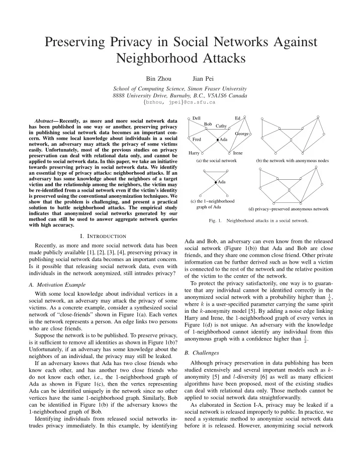
network of “close-friends” shown in Figure 1(a). Each vertex in the network represents a person. An edge links two persons who are close friends. Suppose the network is to be published. To preserve privacy, is it sufficient to remove all identities as shown in Figure 1(b)? Unfortunately, if an adversary has some knowledge about the neighbors of an individual, the privacy may still be leaked. If an adversary knows that Ada has two close friends who know each other, and has another two close friends who do not know each other, i.e., the 1-neighborhood graph of Ada as shown in Figure 1(c), then the vertex representing Ada can be identified uniquely in the network since no other vertices have the same 1-neighborhood graph. Similarly, Bob can be identified in Figure 1(b) if the adversary knows the 1-neighborhood graph of Bob. Identifying individuals from released social networks in- trudes privacy immediately. In this example, by identifying

Ada George (d) privacy−preserved anonymous network graph of Ada (c) the 1−neighborhood (b) the network with anonymous nodes Ada Bob Dell Fred Ed Cathy Irene Harry (a) the social network

• Fig. 1.

Neighborhood attacks in a social network.

Ada and Bob, an adversary can even know from the released social network (Figure 1(b)) that Ada and Bob are close friends, and they share one common close friend. Other private information can be further derived such as how well a victim is connected to the rest of the network and the relative position

• f the victim to the center of the network.

To protect the privacy satisfactorily, one way is to guaran- tee that any individual cannot be identified correctly in the anonymized social network with a probability higher than 1

k,

where k is a user-specified parameter carrying the same spirit in the k-anonymity model [5]. By adding a noise edge linking Harry and Irene, the 1-neighborhood graph of every vertex in Figure 1(d) is not unique. An adversary with the knowledge

• f 1-neighborhood cannot identify any individual from this

anonymous graph with a confidence higher than 1

2.

• B. Challenges

Although privacy preservation in data publishing has been studied extensively and several important models such as k- anonymity [5] and l-diversity [6] as well as many efficient algorithms have been proposed, most of the existing studies can deal with relational data only. Those methods cannot be applied to social network data straightforwardly. As elaborated in Section I-A, privacy may be leaked if a social network is released improperly to public. In practice, we need a systematic method to anonymize social network data before it is released. However, anonymizing social network

data is much more challenging than anonymizing relational data on which most of the previous work focuses. First, it is much more challenging to model the background knowledge of adversaries and attacks about social network data than that about relational data. On relational data, it is of- ten assumed that a set of attributes serving a quasi-identifier is used to associate data from multiple tables, and attacks mainly come from identifying individuals from the quasi-identifier. However, in a social network many pieces of information can be used to identify individuals, such as labels of vertices and edges, neighborhood graphs, induced subgraphs, and their

• combinations. It is much more complicated and much more

difficult than the relational case. Second, it is much more challenging to measure the infor- mation loss in anonymizing social network data than that in anonymizing relational data. Typically, the information loss in an anonymized table can be measured using the sum of information loss in individual tuples. Given one tuple in the

• riginal table and the corresponding anonymized tuple in the

released table, we can calculate the distance between the two tuples to measure the information loss at the tuple level. However, a social network consists of a set of vertices and a set

• f edges. It is hard to compare two social networks by compar-

ing the vertices and edges individually. Two social networks having the same number of vertices and the same number of edges may have very different network-wise properties such as connectivity, betweenness, and diameter. Thus, there can be many different ways to define the measures of information loss and anonymization quality. Last but not least, it is much more challenging to de- vise anonymization methods for social network data than for relational data. Divide-and-conquer methods are extensively applied to anonymization of relational data due to the fact that tuples in a relational table are separable in anonymization. In other words, anonymizing a group of tuples does not affect other tuples in the table. However, anonymizing a social network is much more difficult since changing labels

• f vertices and edges may affect the neighborhoods of other

vertices, and removing or adding vertices and edges may affect other vertices and edges as well as the properties of the network.

• C. Contributions and Organization

Privacy preservation in publishing social networks is a new challenging problem that cannot be solved by one shot. In this paper, we take the initiative to tackle the problem. We identify an essential type of privacy attacks in social networks: neighborhood attacks, which are illustrated in Section I-A. We model the attacks and the anonymization problem systemati- cally, show its difficulty, and develop a practical solution. We conduct an empirical study which indicates that anonymized social networks generated by our method can still be used to answer aggregate network queries with satisfactory accuracy. The rest of the paper is organized as follows. We model neighborhood attacks and review related work in Section II. A practical solution is developed in Section III, and examined empirically using both a real data set and a series of synthetic data sets in Section IV. In Section V, we discuss some

• ther related privacy attacks in social networks as the further

challenges for future work, and also conclude the paper.

• II. PROBLEM DEFINITION AND RELATED WORK

In this section, we first formulate the problem of privacy preserving in social networks by anonymization. Then, we review the related work briefly.

• A. Preliminaries

In this paper, we model a social network as a simple graph G = (V, E, L, L), where V is a set of vertices, E ⊆ V × V is a set of edges, L is a set of labels, and a labeling function L : V → L assigns each vertex a label. For a graph G, V (G), E(G), LG, and LG are the set of vertices, the set of edges, the set of labels, and the labeling function in G, respectively. To keep our discussion simple, we assume that edges do not carry labels. However, our methods can be straightforwardly extended to remove this assumption. The items in the label set L form a hierarchy. For example, if occupations are used as labels of vertices in a social network, L contains not only the specific occupations such as dentist, general physician, optometrist, high school teacher, and primary school teacher, but also general categories like medical doctor, teacher, and professional. We assume that there exists a meta symbol ∗ ∈ L which is the most general category generalizing all labels. For two labels l1, l2 ∈ L, if l1 is more general than l2, we write l1 ≺ l2. For example, medical doctor ≺ optometrist. Moreover, l1 l2 if and only if l1 ≺ l2 or l1 = l2. is a partial order on L. For a graph G and a set of vertices S ⊆ V (G), the induced subgraph of G on S is G(S) = (S, ES, LG, LG) where ES = {(u, v)|(u, v) ∈ E(G) ∧ u, v ∈ S}. In a social network G, the neighborhood of u ∈ V (G) is the induced subgraph of the neighbors of u, denoted by NeighborG(u) = G(Nu) where Nu = {v|(u, v) ∈ E(G)}. Given a graph H = (VH, EH, L, L) and a social network G = (V, E, L, L), an instance of H in G is a tuple (H′, f) where H′ = (VH′, EH′, L, L) is a subgraph in G and f : VH → VH′ is a bijection function such that (1) for any u ∈ VH, L(f(u)) L(u), and (2) (u, v) ∈ EH if and only if (f(u), f(v)) ∈ EH′. Literally, the first condition states that the corresponding labels in H′ can be more general than those in H.

• B. Problem Formulation

To define the problem of privacy preservation in publishing social network data, we need to formulate the following

• issues. First, we need to identify the privacy information

to be preserved. Second, we need to model the background knowledge that an adversary may use to attack the privacy. Last, we need to specify the usage of the published social network data so that an anonymization method can try to retain the utility as much as possible while the privacy information is fully preserved. Different formulations of the above issues may lead to different versions of privacy preservation in social networks.

Here, we propose a version which we believe is useful in many applications. 1) Privacy in Social Networks and Anonymization: In this paper, we are interested in preserving the privacy of individ- uals which are represented as vertices in a social network. Specifically, how a small subset of vertices are connected in a social network is considered as the privacy of those vertices. Consider a social network G = (V, E, L, L) and the anonymization G′ = (V ′, E′, L′, L′) for publishing. We as- sume that no fake vertices are added in the anonymization. That is, there is a bijection function A : V → V ′. This assumption is often desirable in applications since introducing fake vertices may often change the global structure of a social network. Moreover, we assume that for (u, v) ∈ E, (A(u), A(v)) ∈ E′. That is, the connections between vertices in G are retained in G′. For a vertex u ∈ V , if an adversary can identify a vertex u′ ∈ V ′ such that how u connects to other vertices in G is very similar to how u′ connects to other vertices in G′, and is substantially different from how any other vertices connect to others, then the privacy of u is leaked. Therefore, privacy preservation in publishing social network data is to prevent any vertex u ∈ V (G) from being re- identified in G′ with high confidence. Technically, given a positive integer k, G′ preserves the privacy in G if every vertex u ∈ V (G) cannot be re-identified in G′ with a confidence larger than 1

k.

2) Adversary Background Knowledge: In order to attack the privacy of a target individual in the original network, i.e., analyze the released anonymization network and re-identify the vertex, an adversary needs some background knowledge. Equipped with different background knowledge, an adversary may conduct different types of attacks against privacy. There- fore, the assumptions of adversaries’ background knowledge play a critical role in both modeling privacy attacks on social networks and developing anonymization strategies to protect privacy in social network data. In this paper, we assume that an adversary may have the background knowledge about the neighborhood of some target

• individuals. This assumption is realistic in many applications.

Among many types of information about a target victim that an adversary may collect to attack the victim’s privacy, one essential piece of information easy to be collected is the neighborhood, i.e., what the neighbors of the victim are and how the neighbors are connected. Generally, we can consider the d-neighbors of the target vertex, i.e., the vertices within distance d to the target vertex in the network where d is a positive integer. However, when d is large, collecting information about the d-neighbors of a target vertex may often be impractical for an adversary since the adversary may often have a limited access to a large social

• network. Moreover, as found in many social networks, the

network diameter is often small. In other words, when d > 1, an adversary may have to collect information about many

• vertices. Therefore, we confine our discussion in this paper to

the essential case where only the immediate neighbors, i.e., vertices in NeighborG(u), are considered. The case of d > 1 is interesting for future work. An adversary may attack the privacy using the neighbor-

• hoods. For a social network G, suppose an adversary knows

NeighborG(u) for a vertex u ∈ V (G). If NeighborG(u) has k instances in G′ where G′ is an anonymization of G, then u can be re-identified in G′ with confidence 1

k.

Similar to the philosophy in the k-anonymity model [5], to protect the privacy of vertices sufficiently, we want to keep the re-identification confidence lower than a threshold. Let k be a positive integer. For a vertex u ∈ V (G), u is k-anonymous in anonymization G′ if there are at least (k − 1) other vertices v1, . . . , vk−1 ∈ V (G) such that NeighborG′(A(u)), NeighborG′(A(v1)), . . ., NeighborG′(A(vk−1)) are isomor-

• phic. G′ is k-anonymous if every vertex in G is k-anonymous

in G′. Analogous to the correctness of k-anonymity model [5]

• n relational data, we have the following claim.

Theorem 1 (K-anonymity): Let G be a social network and G′ an anonymization of G. If G′ is k-anonymous, then with the neighborhood background knowledge, any vertex in G cannot be re-identified in G′ with confidence larger than 1

k.

An adversary knowing the neighborhood of a target vertex is a strong assumption. Provided privacy is preserved under this assumption, privacy is also preserved when an adver- sary knows only part of the neighborhood (i.e., only some neighbors and some connections among neighbors) of a target vertex. 3) Usage of Anonymized Social Networks: An impor- tant aspect of anonymizing social network data is how the anonymized networks are expected to be used. Different ap- plications may have different expectations. In some situations, anonymized networks may be used to analyze the global struc-

• tures. In some other situations, anonymized networks may be

used to analyze the micro-structures. Clearly, different usage expectations may lead to different anonymization schemes. In this paper, we focus on using anonymized social networks to answer aggregate network queries. An aggregate network query computes the aggregate on some paths or subgraphs satisfying some given conditions. As an example, suppose a user is interested in the average distance from a medical doctor vertex to a teacher vertex in a network. For each doctor vertex, we can find the nearest neighbor vertex that is a teacher. Then, the aggregate network query returns the average of the distance between a doctor vertex to its nearest teacher neighbor. Aggregate network queries are useful in many applica- tions, such as customer relationship management. While many types of queries on social networks are interesting, we are particularly interested in aggregate network queries in this paper since typically detail data is needed to answer such queries accurately. Using aggregate network queries we can examine the effectiveness of social network anonymization in a meaningful way. 4) Problem Definition and Complexity: Given a social network G, we want to compute an anonymization G′ such that (1) G′ is k-anonymous; (2) each vertex in G is anonymized to a vertex in G′ and G′ does not contain any fake vertex; (3) every edge in G is retained in G′; and (4) G′ can be used to answer aggregate network queries as accurately as possible.

To understand the difficulty of the problem, we consider a simple case where all vertices in G carry the same label, or equivalently, G is not labeled. Theorem 2 (Complexity): The following k-anonymity prob- lem in social network is NP-hard. Instance: a social network G = (V, E, L, L) where L = ∗ and ∀u ∈ V , L(u) = ∗, positive integers k and n. Question: is there an anonymized social network G′ = (V, E′, L, L) such that E ⊂ E′, |E′ − E| = n, and G′ is k-anonymous? Proof sketch. The proof is constructed by reducing the NP- hard k-DIMENSIONAL PERFECT MATCHING problem [7] to the k-anonymity problem in social networks. Limited by space, we omit the details here.

• C. Related Work

Privacy becomes a more and more serious concern in many

• applications. The development of techniques that incorporate

privacy concerns has become a fruitful direction for database and data mining research. One of the privacy concerned problems is publishing mi- crodata for public use [8], which has been extensively studied

• recently. A large category of privacy attacks is to re-identify

individuals by joining the published table with some external tables modeling the background knowledge of users. To battle this type of attacks, the mechanism of k-anonymity was proposed in [9], [5]. Specifically, a data set is said to be k- anonymous (k ≥ 1) if, on the quasi-identifier attributes (i.e., the minimal set of attributes in the table that can be joined with external information to re-identify individual records), each record is indistinguishable from at least k − 1 other records within the same data set. The larger the value of k, the better the privacy is protected. Machanavajjhala et al. [6] showed that a k-anonymized dataset has some subtle but severe privacy problems due to the lack of diversity in the sensitive attributes. In particular, they showed that, the degree of privacy protection does not really depend on the size of the quasi-identifier attribute set. Instead, it is determined by the number of distinct sensitive values associated with each quasi-identifier attribute set. The

• bservation leads to the notion of l-diversity [6]. [10] proved

that l-diversity always guarantees stronger privacy preservation than k-anonymity. In this paper, we focus on k-anonymity since k-anonymity is the most essential and most applicable privacy model, which can be used even when sensitive attributes are not defined. A few governmental privacy regulations including HIPAA and European Union Data Directive adopted k-anonymity. Beyond microdata, some other data sources such as social network data also have privacy concerns when they are pub- lished for public use. Typically, social network data can be represented as a graph, in which vertices correspond to people

• r other social entities, and edges correspond to social links

between them [11]. As a first step to hide information about social entities while preserving the global network proper- ties, the released social network data has to go through the anonymization procedure which replaces social entity names with meaningless unique identifiers [12]. Although this kind of anonymization can exactly preserve the unannotated structure

• f the social network, it may still leak a lot of information.

Attacks in social network data can be regarded as one kind of link mining [13]. Specifically, as a pioneer work about privacy in social network data, Backstrom et al. [12] described a family of attacks based on random graph theory. For example, an attacker may plant some well constructed sub- structures associated with the target entities in advance. Once the social network data is collected and published, the attacker can first try to identify the planted structures and thus peek the linkage between the target vertices. However, there is no practical solution proposed in [12] to counter those attacks. The attacks proposed in [12] are different from the neigh- borhood attacks addressed in this paper. The attacks in [12] need to plant a set of deliberative structures before the social network data is anonymized, which is a task hard to achieve in some situations. As shown before, even without planting deliberative structures, the released social network data is still in danger, as neighborhood attacks are still possible. Wang et al. [14] adopted description logic as the underly- ing knowledge representation formalism, and proposed some metrics of anonymity for assessing the risk of breaching confidentiality by disclosing social network data. However, they did not give any anonymization algorithms for social network data. Simultaneous to our study, Hay et al. [15] presented a framework for assessing the privacy risk of sharing anonymized network data. They modeled the adversaries’ background knowledge as vertex requirement structural queries and subgraph knowledge structural queries, and pro- posed a privacy requirement k-candidate anonymity which is similar to k-anonymity in tabular data. They developed a random graph perturbation method by randomly deleting or adding edges to anonymize a social network. Their model assumes that the nodes and the edges in a social network are not labeled. Recently, Zheleva et al. [16] proposed a model different from ours. They focused on social networks where nodes are not labeled but edges are labeled. Some types of edges are sensitive and should be hidden. They provided the edge anonymization methods based on edge clustering and removal to prevent link re-identification.

• III. AN ANONYMIZATION METHOD

In this section, we introduce a practical method to anonymize a social network to satisfy the k-anonymity re-

• quirement. The method is in two steps.

First, we extract the neighborhoods of all vertices in the

• network. To facilitate the comparisons among neighborhoods
• f different vertices including the isomorphism tests which will

be conducted frequently in anonymization, we propose a sim- ple yet effective neighborhood component coding technique to represent the neighborhoods in a concise way. In the second step, we greedily organize vertices into groups and anonymize the neighborhoods of vertices in the same

• group. Due to the well recognized power law distribution of

v1 v5 NeighborG(u) v2 v4 v3 v6 u

C3 C1

C2

• Fig. 2.

Neighborhood and neighborhood components (the dashed edges are just for illustration and are not in the neighborhood subgraph). x x z y v3 v2 v1 v0 y z x x v3 v2 v0 v1 y z x x

(a) Graph G (b) DFS-tree T1 (c) DFS-tree T2

• Fig. 3.

DFS codes, starting from different vertices.

the degrees of vertices in large social networks, we start with those vertices of high degrees.

• A. Neighborhood Extraction and Coding

In order to meet the k-anonymity requirement, we need to put vertices into groups and anonymize the neighborhoods of vertices in a group. Ideally, vertices having similar neighbor- hoods should be grouped together. As the first step, we extract neighborhoods of vertices and represent them in a concise way. Extracting the neighborhood of a vertex is straightforward. The challenge is how we can represent the neighborhood information to facilitate the later operations in anonymization. Since we need to anonymize all neighborhoods of the vertices in one group to the same, isomorphism tests are frequently conducted. The general graph isomorphism problem which determines whether two graphs are isomorphic is NP-hard [17]. Here, we propose a coding technique for neighborhood subgraphs so that whether two neighborhoods are isomorphic can be determined by the corresponding coding. In a social network G, a subgraph C of G is a neighborhood component of u ∈ V (G) if C is a maximal connected subgraph in NeighborG(u). Example 1 (Neighborhood component): Figure 2 shows NeighborG(u), the neighborhood

• f

a vertex u. NeighborG(u) contains three neighborhood components, C1, C2, and C3 as shown in the figure. Clearly, the neighborhood of a vertex can be divided into neighborhood components. To code the whole neighborhood, we need to first code each component. The depth-first search tree (DFS-tree for short) [18] is popularly used for navigating connected graphs. Thus, it is natural to encode the edges and vertices in a graph based on its DFS-tree. All the vertices in G can be encoded in the pre-

• rder of T. However, the DFS-tree is generally not unique for a
• graph. That is, there can be multiple DFS-trees corresponding

to a given graph. For example, Figures 3(b) and 3(c) show two DFS-trees of the graph G in Figure 3(a). The thick edges in Figures 3(b) and 3(c) are those in the DFS-trees, and are called the forward edges, while the thin edges are those not in the DFS- trees, and are called the backward edges. The vertices in the graph are encoded v0 to v3 according to the pre-order of the corresponding DFS-trees. To solve the uniqueness problem, a minimum DFS code notation is proposed in [19]. For any connected graph G, let T be a DFS-tree of G. Then, an edge is always listed as (vi, vj) such that i < j. A linear order ≺ on the edges in G can be defined as follows. Given edges e = (vi, vj) and e′ = (vi′, vj′). e ≺ e′ if (1) when both e and e′ are forward edges (i.e., in DFS-tree T), j < j′ or (i > i′ ∧ j = j′); (2) when both e and e′ are backward edges (i.e., edges not in DFS-tree T), i < i′ or (i = i′ ∧ j < j′); (3) when e is a forward edge and e′ is a backward edge, j ≤ i′; or (4) when e is a backward edge and e′ is a forward edge, i < j′. For a graph G and a DFS-tree T, a list of all edges in E(G) in order ≺ is called the DFS code of G with respect to T, denoted by code(G, T). For example, the DFS code with respect to the DFS-tree T1 in Figure 3(b) is code(G, T1) = (v0, v1, x, x)-(v1, v2, x, z)-(v2, v0, z, x)- (v1, v3, x, y), where an edge (vi, vj) is written as (vi, vj, L(vi), L(vj)), i.e., the labels are included. Similarly, the DFS code with respect to the DFS-tree T2 in Figure 3(c) is code(G, T2) = (v0, v1, y, x)-(v1, v2, x, x)-(v2, v3, x, z)- (v3, v1, z, x). Suppose there is a linear order over the label set L. Then, for DFS-trees T1 and T2 on the same graph G, their DFS codes can be compared lexically according to the vertex pairs as labels of edges. For example, we have code(G, T1) < code(G, T2) in Figures 3(b) and 3(c). The lexically minimum DFS code is selected as the repre- sentation of the graph, denoted by DFS(G). In our example in Figure 3, DFS(G) = code(G, T1). Minimum DFS code has a nice property [19]: two graphs G and G′ are isomorphic if and only if DFS(G) = DFS(G′). Using minimum DFS code, we can code every component of the neighborhood of a vertex. Now, the problem becomes how we can combine the minimum DFS codes of all components in a neighborhood into one code. For two neighborhood components Ci and Cj in NeighborG(u), we define Ci ≺ Cj if (1) |V (Ci)| < |V (Cj)|;

• r (2) |V (Ci)| = |V (Cj)| and |E(Ci) < |E(Cj)|; or (3)

|V (Ci)| = |V (Cj)|, |E(Ci) = |E(Cj)|, and DFS(Ci) is smaller than DFS(Cj). Based on the neighborhood component order, we can assign a canonical label for each neighborhood. In a so- cial network G, for vertex u ∈ V (G), the neigh- borhood component code of NeighborG(u) is a vector NCC(u) = (DFS(C1), . . . , DFS(Cm)) where C1, . . . , Cm are the neighborhood components of NeighborG(u), i.e., NeighborG(u) = ∪m

i=1Ci, Ci Cj for 1 ≤ i < j ≤ m.

Example 2 (Neighborhood component code): In Figure 2, the neighborhood component code of NeighborG(u) is NCC(u) = (DFS(C1), DFS(C2), DFS(C3)).

Using neighborhood component code, we can easily identify isomorphic neighborhoods. Theorem 3 (Neighborhood component code): For two ver- tices u, v ∈ V (G) where G is a social network, NeighborG(u) and NeighborG(v) are isomorphic if and only if NCC(u) = NCC(v). Using neighborhood component code to label and index neighborhoods has some advantages. First, it is easy to ex- amine whether a group of neighborhoods are isomorphic. Second, since each neighborhood is decomposed into several neighborhood components, it is easy to calculate the structure similarity between two neighborhoods. Third, we can find sim- ilar components between two neighborhoods. Anonymizing similar components can lead to low information loss and high similarity between the anonymization and the original social network.

• B. Social Network Anonymization

One major challenge in anonymizing a social network is that changing labels of vertices and adding edges may affect the neighborhoods of some other vertices as well as the properties

• f the network. It has been well recognized that the following

two properties often hold in practical social networks. The properties help us in designing anonymization methods. Property 1: vertex degree in power law distribution. The degrees of vertices in a large social network often follow the power law distribution [20]. Such degree distributions have been identified in various social networks including Internet, biological networks, and co-authorship networks. Property 2: the “small-world phenomenon” [11]. It is also popularly known as “six degrees of separation”, which states that large social networks in practice often have surprisingly small average diameters. Our social network anonymization method processes ver- tices in the degree descending order, and utilizes the above two properties of large social networks in practice. The k-anonymity requires that each vertex u ∈ V (G) is grouped with at least (k − 1) other vertices such that their anonymized neighborhoods are isomorphic. For a group S of vertices having the isomorphic anonymized neighborhoods, all vertices in S have the same degree. Since the degrees

• f vertices in a large social network follow a power law

distribution, only a small number of vertices have a high

• degree. Processing those vertices of high degrees first can

keep the information loss about those vertices low. There are

• ften many vertices of a low degree. It is relatively easy to

anonymize those low degree vertices and retain high quality. Moreover, as will be shown soon, low degree vertices can be used to anonymize those high degree vertices and do not affect the diameters of the network too much. 1) Anonymization Quality Measure: In our social network anonymization model, there are two ways to anonymize the neighborhoods of vertices: generalizing vertex labels and adding edges. Each of the two methods leads to some in- formation loss. The information loss due to generalization of vertex labels can be measured by the normalized certainty penalty [21]. Consider a vertex u of label l1, where l1 is at the leaf level

• f the label hierarchy, i.e., l1 does not have any descendant.

Suppose l1 is generalized to l2 for u where l2 ≺ l1. Let size(l2) be the number of descendants of l2 that are leafs in the label hierarchy, and size(∗) be the total number of leafs in the label hierarchy. Then, the normalized certainty penalty

• f l2 is NCP(l2) = size(l2)

size(∗) .

The information loss due to adding edges can be measured by the total number of edges added and the number of vertices that are not in the neighborhood of the target vertex and are linked to the anonymized neighborhood for the purpose of anonymization. Consider two vertices u1, u2 ∈ V (G) where G is a social

• network. Suppose NeighborG(u1) and NeighborG(u2) are

generalized to NeighborG′(A(u1)) and NeighborG′(A(u2)) such that NeighborG′(A(u1)) and NeighborG′(A(u2)) are

• isomorphic. Let H

= NeighborG(u1) ∪ NeighborG(u2) and H′ = NeighborG′(A(u1)) ∪ NeighborG′(A(u2)). The anonymization cost is Cost(u, v) = α ·

v′∈H′ NCP(v′)

+β · |{(v1, v2)|(v1, v2) ∈ E(H), (A(v1), A(v2)) ∈ E(H′)}| +γ · (|V (H′)| − |V (H)|) where α, β and γ are the weights specified by users. Lit- erally, the cost consists of three parts. The first part is the normalized certainty penalty measuring the information loss

• f generalizing labels of vertices. The second part measures

the information loss due to adding edges. The last part counts the number of vertices that are linked to the anonymized neighborhoods to achieve k-anonymity. The anonymization cost of two vertices u and v measures the similarity between NeighborG(u) and NeighborG(v). The smaller the anonymization cost, the more similar the two neighborhoods. 2) Anonymizing Two Neighborhoods: Now, let us con- sider a greedy method to anonymize two neighborhoods NeighborG(u) and NeighborG(v). We first find all perfect matches of neighborhood compo- nents in NeighborG(u) and NeighborG(v). Two components perfectly match each other if they have the same minimum DFS code. Those perfect matches are marked as “matched” and pass over for further consideration. For example, consider two vertices u and v whose neigh- borhoods are shown in Figure 4. Each vertex is shown in the form of (id, label). The neighborhood component C2(u) ∈ NeighborG(u) perfectly matches C3(v) ∈ NeighborG(v). For those unmatched components, the anonymization al- gorithm tries to pair similar components and anonymize

• them. The similarity between two components is based on

the anonymization cost. To calculate the similarity between two components, we try to match similar vertices in the two components as much as possible. This is a traditional substructure similarity search problem, which has been proved NP-hard [22]. Instead of computing the optimal matching, we conduct a greedy match. To start with, we first try to find two vertices with the same degree and the same label in the two components to be

(v6, l5) (v1, l2) (v2, l5) (v3, l1) (v4, l2) (v5, l1) (v7, l1) (v8, l2) C1(v) C2(v) C3(v) NeighborG(v) (s2, l7) (s1, l2) (s3, l1) (s4, l4) (s5, l6) (s7, l5) (s6, l1) (s8, l1) (s9, l2) C1(s) C2(s) C3(s) Anonymized neighborhood (u4, l4) (u2, l4) (u5, l1) (u6, l2) (u7, l1) (u8, l3) C1(u) C2(u) C3(u) (u1, l2) (u3, l1) ∗ l6 l7 (w1, l4) (w2, l5) NeighborG(u) New neighbor nodes Label hierarchy l5 l4 l3 l2 l1

• Fig. 4.

Anonymizing two neighborhoods.

• matched. If there are multiple matching vertex pairs, the pair

with the highest vertex degree is chosen. If there is no such a pair of matching vertices, we relax the matching requirement (vertex degree and label), calculate the difference of degrees and the normalized certainty penalty of generalizing the labels in the label hierarchy, and choose the one with the minimum anonymization cost. Then, we conduct a breadth-first search to match vertices one by one, until all possible vertex matchings are found. The anonymization cost is calculated according to the matching, and is used to measure the similarity of the two components. Consider components C1(u) and C1(v) in Figure 4. Vertices u1 and v1 match. We start from these two vertices and conduct a breadth-first search. Vertex v2 partially matches vertex u2. Vertex v3 partially matches vertex u3. The vertex matching stops since all possible vertex matchings are found. However, vertex u4 does not find any vertex matching in C1(v). Thus we have to find a vertex w1 ∈ V (G) that is neither in C1(v) nor in C1(u), and add it into C1(v), so that C1(u) and C1(v) can be anonymized to the same. When a vertex has to be introduced into the neighborhood for the sake of anonymization, the following rules are used: we first consider those vertices in V (G) that are unanonymized. The vertex with smallest degree has the highest priority. If there are more than one candidate with the same smallest degree, we choose the one having the closest label in terms of normalized certainty penalty. If we cannot find any other ver- tex that is unanonymized, we select one anonymized vertex w with the smallest degree and satisfying the label requirement, and mark w and its (k − 1) other vertices anonymized in the same group as “unanonymized”. In our example, suppose we can find an unanonymized vertex (w1, l4) to be added to C1(u), the anonymization cost of C1(u) and C1(v) is α·

• v′∈V (C1(u))∪V (C1(v))

NCP(L(A(v′))+ β · 1 + γ · 1 = α · 4 5 + β + γ.

Input: a social network G = (V, E), the anonymization requirement parameter k, the cost function parameters α, β and γ; Output: an anonymized graph G′; Method: 1: initialize G′ = G; 2: mark vi ∈ V (G) as “unanonymized”; 3: sort vi ∈ V (G) as VertexList in neighborhood size descending

• rder;

4: WHILE (VertexList = ∅) DO 5: let SeedVertex = VertexList.head() and remove it from VertexList; 6: FOR each vi ∈ VertexList DO 7: calculate Cost(SeedVertex, vi) using the anonymization method for two vertices; END FOR 8: IF (VertexList.size() ≥ 2k − 1) DO let CandidateSet contain the top k − 1 vertices with the smallest Cost; 9: ELSE 10: let CandidateSet contain the remaining unanonymized vertices; 11: suppose CandidateSet= {u1, . . . , um}, anonymize Neighbor(SeedVertex) and Neighbor(u1) as discussed in Section III-B.2; 12: FOR j = 2 to m DO 13: anonymize Neighbor(uj) and {Neighbor(SeedVertex), Neighbor(u1), . . . ,Neighbor(uj−1)} as discussed in Section III-B.2, mark them as “anonymized”; 14: update VertexList; END FOR END WHILE

• Fig. 5.

Anonymizing a Social Network.

Based on the component similarity, we can pair similar

• components. We start with the component with the largest

number of vertices. This component is paired with the most similar component in the other neighborhood. The two paired components are anonymized to the same, marked “matched”, and removed from consideration. The matching continues until all components in one neighborhood are marked “matched”. If there are some components left in the other neighborhood say NeighborG(u), we use some other vertices in V (G) that are not in NeighborG(u) to construct a component and add it to NeighborG(u) to construct the matching and anonymiza-

• tion. The vertices are selected using the same criteria as

selecting vertices to match two components. We anonymize each pair of matched neighborhood com- ponents to the same. The two neighborhoods then are

• anonymized. For example, in Figure 4, the algorithm matches

components C1(u) and C1(v), and C2(v) and C3(u) in turn. As a result, two vertices w1 and w2 from V (G) have to be added into components C1(v) and C3(u), respectively. 3) Anonymizing a Social Network: We propose a greedy method to anonymize a social network as shown in Figure 5. First, we mark all vertices in the network as “unanonymized”. We maintain a list VertexList

• f

“unanonymized” vertices in the neighborhood size descending

• rder: for vertices u, v

∈ V (G), if |V (NeighborG(u))| < |V (NeighborG(v))|,

• r

|V (NeighborG(u))| = |V (NeighborG(v))| and |E(NeighborG(u))| <

|E(NeighborG(v))|, then v precedes u in the list. If their neighborhoods have the same numbers of vertices and edges, they can be ordered arbitrarily. Iteratively, we pick the first vertex SeedVertex in the list

• VertexList. The anonymization cost of SeedVertex and any
• ther vertices in VertexList is calculated using the anonymiza-

tion method for two vertices discussed in Section III-B.2. If the number of unanonymized vertices in VertexList is at least 2k − 1, we select a set CandidateSet of the top k − 1 vertices in VertexList with the smallest anonymization cost. We can easily give a lower bound of the anonymization cost based on the number of vertices and the number of edges in two neighborhoods. Since all vertices in VertexList have a neighborhood size smaller than or equal to that of SeedVertex, we scan VertexList in the neighborhood size descending order, and stop once the lower bound of the anonymization cost exceeds the cost of the current (k − 1)-th most similar vertex. The SeedVertex and the vertices in CandidateSet= {u1, . . . , um} are anonymized in turn using the anonymization method for two vertices discussed in Section III-B.2. The anonymization of SeedVertex and u1 is straightforward. After these two vertices are anonymized, their neighborhoods are

• identical. When we anonymize them with respect to u2, any

change (e.g., adding an edge or a neighbor node) to the neighborhood of SeedVertex will be applied to u1 as well, so that the neighborhoods of SeedVertex, u1 and u2 are anonymized to the same. The process continues until the neighborhoods of SeedVertex and u1, . . . , um are anonymized. During the anonymization of a group of vertices, some changes may occur to some other vertices v that have been marked as “anonymized” in another group (e.g., adding edges between an anonymized vertex and a vertex being anonymized based on vertex matching). In order to maintain the k- anonymity for those vertices, we apply the same changes to every other k−1 vertices having the isomorphic neighborhoods as v. Once those k vertices are changed, they are marked as “unanonymized” and inserted into the VertexList again. When the number of unanonymized vertices in VertexList is less than 2k, to satisfy the k-anonymity, the remaining vertices in VertexList have to be considered together in anonymization. They are added to CandidateSet in a batch. The social network anonymization algorithm continues until all the vertices in the graph are marked as “anonymized”. Theorem 4 (Termination): The algorithm in Figure 5 termi- nates for a finite social network of at least k vertices. Proof sketch. Clearly, a clique of n vertices where each vertex is labeled ∗ is k-anonymous provided n ≥ k. In each iteration such that VertexList is not shortened, the algorithm either adds some edges into the network, or generalizes the labels of some vertices towards ∗. In the worst case, the network will be anonymized to a clique. Surprisingly, as shown in our experiments, the algorithm can stop very quickly in practice, and the anonymization cost is relatively small. This is due to the two important properties of real social networks (vertex degree in power law distribution and small world phenomenon). Using different synthetic data sets, we find that most of the time we do not

k Removing labels Generalizing to affiliations 5 1.3% 12.7% 10 3.9% 16.1% 15 7.1% 19.4% 20 12.0% 23.2% TABLE I THE PERCENTAGES OF VERTICES VIOLATING k-ANONYMITY IN THE

CO-AUTHORSHIP DATA.

need to anonymize the remaining vertices that are less than 2k, since they have the same labels, very low degree (1 in many sparse social networks), and isomorphic neighborhoods.

• IV. EMPIRICAL EVALUATION

In this section, we report a systematic empirical study to evaluate our anonymization method using both real data sets and synthetic data sets. All the experiments were conducted

• n a PC computer running the Microsoft Windows XP SP2

Professional Edition operating system, with a 3.0 GHz Pen- tium 4 CPU, 1.0 GB main memory, and a 160 GB hard disk. The program was implemented in C/C++ and was compiled using Microsoft Visual Studio .NET 2005.

• A. Neighborhood Attacks in Real Data

We used a real co-authorship data set from KDD Cup 2003 to examine whether neighborhood attacks may happen in

• practice. The data set was from the e-print arXiv (arXiv.org),

and contains a subset of papers in the high-energy physics section of the arXiv. The L

AT

EX sources of all papers are

• provided. We extracted author names from the data sources

and constructed a co-authorship graph. Each vertex in the graph represents an author, and two vertices are linked by an edge if the two corresponding authors co-authored at least one paper in the data set. There are 57, 448 vertices and 120, 640 edges in the co-authorship graph and the average number of vertex degrees is about 4. We tested two ways to preserve the privacy of authors by generalizing labels. In the first method, we removed all labels, i.e., author names. In the second method, we use the author’s affiliation as the label, i.e., all authors from the same institution have the same label. After generalization, for each vertex, we extracted its neighborhood and counted the number of other vertices in the graph that have the isomorphic

• neighborhoods. Table I shows the percentages of vertices

whose neighborhoods violate the k-anonymity. Table I clearly shows that the neighborhood attacks are a real issue for social network data publishing. When the value

• f k increases, the number of vertices violating k-anonymity
• increases. Moreover, the more specific are the vertex labels,

the more vertices fail the k-anonymity. Anonymizing labels

• nly cannot prevent neighborhood attacks effectively.
• B. Anonymization Performance

We use the R-MAT graph model [23] to generate synthetic data sets. R-MAT can generate graphs with power law vertex degree distribution and small-world characteristic, which are

100 200 300 400 500 600 700 800 900 1000 5000 10000 15000 20000 25000 # dummy edges Number of vertices k=5 k=10 k=15 k=20 500 1000 1500 2000 2500 3000 3500 4000 4500 5000 5000 10000 15000 20000 25000 NCP Number of vertices k=5 k=10 k=15 k=20

average vertex degree = 3

1000 1500 2000 2500 3000 3500 5000 10000 15000 20000 25000 # dummy edges Number of vertices k=5 k=10 k=15 k=20 1000 2000 3000 4000 5000 6000 7000 8000 9000 5000 10000 15000 20000 25000 NCP Number of vertices k=5 k=10 k=15 k=20

average vertex degree = 7

• Fig. 7.

Anonymization cost on various synthetic data sets.

1200 1220 1240 1260 1280 1300 1320 0.8 0.9 1 1.1 1.2 # dummy edges gamma alpha=90 alpha=100 alpha=110 3180 3200 3220 3240 3260 3280 3300 3320 3340 0.8 0.9 1 1.1 1.2 NCP gamma alpha=90 alpha=100 alpha=110

• Fig. 6.

The effect of parameters in anonymization quality measure.

the two most important properties for many real-world social networks. R-MAT takes 4 probability parameters, namely a, b, c and d. Consider the adjacency matrix representation A of the graph. Assume that each element aij in A is non-zero if there exists an edge between vertices i and j. Given the number of vertices n and the number of edges m, R-MAT starts with an empty n×n adjacency matrix A. It recursively divides the adjacency matrix into four equal-size partitions, and distributes edges within these partitions with a set of unequal probabilities. Each edge chooses one of the four partitions with probabilities a, b, c and d, respectively, such that a + b + c + d = 1. The parameters a, b, c and d can be determined based on the required community structure and vertex degree distribution, as detailed in [23]. The study [23] conjectures that the ratios a/b and a/c are approximately 3/1 in many real world graphs, and a ≥ d. We used the default values of 0.45, 0.15, 0.15 and 0.25 for those four parameters, respectively. We generated a series

• f synthetic data sets by varying the number of vertices from

5, 000 to 25, 000 and the average vertex degree from 3 to 7. Hereafter, we refer to a synthetic data set as D(n, d), where n and d are the number of vertices and the average vertex degree,

• respectively. The edge weight was set in the range [0, 100] by
• default. We assigned each vertex a label based on its average

edge weight. A simple two level hierarchy structure for those labels was generated. We first examined the effect of parameters α, β and γ in the anonymization quality measure. β was set to 1 as the base. We changed the values of α and γ, and measured the number

• f edges added and the normalized certainty penalty incurred

in the anonymized graphs. The results for data set D(15K, 5) and k = 10 are shown in Figure 6. The results show that we can trade off between adding edges and generalizing labels by tuning the three parameters. Often adding less edges is more desirable in anonymizing a social network since the network structures can be preserved better. We observed that, on the synthetic data sets, when α = 100 and γ = 1.1, the number

• f edges added is small and the normalized certainty penalty

is moderate. Hereafter, we use 100, 1, and 1.1 as the default

50 100 150 200 250 300 350 5000 10000 15000 20000 25000 Running time (sec) Number of vertices k=5 k=10 k=15 k=20

average vertex degree = 3

50 100 150 200 250 300 350 400 450 5000 10000 15000 20000 25000 Running time (sec) Number of vertices k=5 k=10 k=15 k=20

average vertex degree = 7

• Fig. 8.

The runtime on various synthetic data sets.

values for α, β and γ. Figure 7 reports the anonymization quality on various synthetic data sets with respect to different k values, and shows the anonymization cost in both the number of edges added and the normalized certainty penalty. First, when the number of vertices increases, the anonymization cost increases. However, the increase of the number of edges added is sub- linear, since in a larger network it is more likely to find similar

• neighborhoods. Second, when k increases, the anonymization

cost also increases, because more neighborhoods need to be anonymized in a group. Last, when the average number of vertex degree increases, the anonymization cost increases, too. In a denser network, the neighborhoods are more diverse and more edges are needed to anonymize different neighborhoods. Figure 8 shows the runtime on various synthetic data sets with respect to different k values. The runtime increases when the average vertex degree increases, since the network becomes denser. Moreover, the larger the k, the longer the runtime since more neighborhoods in a group need to be anonymized.

• C. Anonymizing the Co-authorship Data Set

We built a 3-level label hierarchy for the KDD cup 2003 co-authorship data set. The leaf vertices are those labels with author affiliations. The middle level contains the countries

• f the authors’ affiliations. The root is the most general

label ∗. We anonymized the co-authorship data set using

• ur anonymization method. The number of edges added, the

normalized certainty penalty and the runtime with different values of k are shown in Figure 9. Comparing to the total number of edges in the data set (120, 640), the number of edges added is less than 6% even when k = 20. Moreover, the runtime is scalable with respect to k.

• D. Aggregate Query Answering

To test the utility of the anonymized social networks, we conducted aggregate network queries on the KDD Cup 2003 co-authorship data set, and the anonymized networks. For two labels l1 and l2 in the data set, we calculated the average

1000 2000 3000 4000 5000 6000 7000 5 10 15 20 # dummy edges k 2000 4000 6000 8000 10000 12000 14000 5 10 15 20 NCP k 300 400 500 600 700 800 900 5 10 15 20 Running time (sec) k

• Fig. 9.

Anonymizing the KDD cup 2003 co-authorship data set.

2 4 6 8 10 5 10 15 20 Error rate (%) k

• Fig. 10.

Query answering on the KDD Cup 2003 co-authorship data set.

distance from a vertex with label l1 to its nearest vertex with label l2. Since labels are organized in a hierarchy structure, when we calculated the average distance, we also considered distance from vertices with labels l′

1 to vertices with labels l′ 2

such that l1 l′

1 and l2 l′

• 2. The error rate is d−d′

d , where d

and d′ are the average distances in the original network and in the anonymized network, respectively. We randomly picked 10 label pairs from the label hierarchy, and calculated the average error rate of them. The results are shown in Figure 10. After the anonymization, with some edges added, the average distance decreases. Therefore, the error rate is always positive. However, the error rate is small even when k is up to 20, since the number of edges added is small, as shown in Figure 9.

• V. DISCUSSION AND CONCLUSIONS

In this paper, we tackled the novel and important problem

• f preserving privacy in social network data, and took an

initiative to combat neighborhood attacks. We modeled the problem systematically and developed a practically feasible

• approach. An extensive empirical study using both a real data

set and a series of synthetic data sets strongly indicated that neighborhood attacks are real in practice, and our method is highly feasible. Moreover, anonymized social networks can still be used to answer aggregate queries accurately. As social network data is much more complicated than relational data, privacy preserving in social networks is much more challenging and needs many serious efforts in the fu-

• ture. Particularly, modeling adversarial attacks and developing

privacy preservation strategies are critical. For future work, we believe that the following two types of attacks should be addressed systematically. We only handle 1-neighborhoods in this paper. It is very interesting and could be desirable in some applications that d-neighborhoods (d > 1) are protected. However, this will introduce a serious challenge in computation. The neighbor- hood size increases exponentially as d increases. Isomorphism tests and anonymization of large neighborhoods are very challenging. A k-anonymous social network still may leak privacy. If an adversary can identify a victim in a group of vertices anonymized in a group, but all are associated with some sensitive information, then the adversary still can know that sensitive attribute of the victim. Some mechanism analogous to l-diversity [6] should be introduced. ACKNOWLEDGMENT The research is supported in part by an NSERC Discovery

• Grant. All opinions, findings, conclusions and recommen-

dations in this paper are those of the authors and do not necessarily reflect the views of the funding agencies. We are grateful to Dr. Yufei Tao and the anonymous review- ers for their informative comments which help to improve the quality of the paper. REFERENCES

[1] L. Adamic and E. Adar, “How to search a social network,” Social Networks, vol. 27, no. 3, pp. 187–203, July 2005. [2] G. Kossinets and D. J. Watts, “Empirical analysis of an evolving social network,” Science, vol. 311, no. 5757, pp. 88–90, January 2006. [3] L. Backstrom et al., “Group formation in large social networks: mem- bership, growth, and evolution,” in KDD’06. [4] R. Kumar et al., “Structure and evolution of online social networks,” in KDD’06. [5] L. Sweeney, “K-anonymity: a model for protecting privacy,” Interna- tional Journal on uncertainty, Fuzziness and Knowledge-based System,

• vol. 10, no. 5, pp. 557–570, 2002.

[6] A. Machanavajjhala et al., “L-diversity: Privacy beyond k-anonymity,” in ICDE’06. [7] E. Hazan et al., “On the complexity of approximating k-dimensional matching,” in Approximation, Randomization, and Combinatorial Opti-

• mization. Algorithms and Techniques, 2003, pp. 83–97.

[8] P. Samarati, “Protecting respondents’ identities in microdata release,” IEEE Transactions on Knowledge and Data Engineering, vol. 13, no. 6,

• pp. 1010–1027, 2001.

[9] P. Samarati and L. Sweeney, “Generalizing data to provide anonymity when disclosing information,” in PODS’98. [10] X. Xiao and Y. Tao, “Personalized privacy preservation,” in SIG- MOD’06. [11] S. Wasserman and K. Faust, Social Network Analysis. Cambridge University Press, 1994. [12] L. Backstrom et al., “Wherefore art thou r3579x?: anonymized social networks, hidden patterns, and structural steganography,” in WWW’07. [13] L. Getoor and C. P. Diehl, “Link mining: a survey,” ACM SIGKDD Explorations Newsletter, vol. 7, no. 2, pp. 3–12, 2005. [14] D.-W. Wang et al., “Privacy protection in social network data disclo- sure based on granular computing,” in Proceedings of the 2006 IEEE International Conference on Fuzzy Systems, 2006, pp. 997–1003. [15] M. Hay et al., “Anonymizing social networks,” University of Mas- sachusetts Amherst, Tech. Rep. 07-19, 2007. [16] E. Zheleva and L. Getoor, “Preserving the privacy of sensitive relation- ships in graph data,” in PinKDD’07. [17] M. R. Garey and D. S. Johnson, Computers and Intractability: A Guide to the Theory of NP-Completeness. New York, NY, USA: W. H. Freeman & Co., 1979. [18] T. H. Cormen et al, Introduction to Algorithms, Second Edition. MIT Press and McGraw-Hill, 2002. [19] X. Yan and J. Han, “gspan: Graph-based substructure pattern mining,” in ICDM’02. [20] M. Faloutsos et al., “On power-law relationships of the internet topol-

• gy,” in SIGCOMM’99.

[21] J. Xu et al., “Utility-based anonymization using local recoding,” in KDD’06. [22] X. Yan et al., “Graph indexing: a frequent structure-based approach,” in SIGMOD’04. [23] D. Chakrabarti et al., “R-mat: A recursive model for graph mining,” in SDM’04.