} Probability hot rain 0.1 ? sun 0.6 Distribution cold sun - - PDF document

1

CSE 473: Artificial Intelligence Probability

Dieter Fox University of Washington

[These slides were created by Dan Klein and Pieter Abbeel for CS188 Intro to AI at UC Berkeley. All CS188 materials are available at http://ai.berkeley.edu.]

Topics from 30,000’

§ We’re done with Part I Search and Planning! § Part II: Probabilistic Reasoning

§ Diagnosis § Speech recognition § Tracking objects § Robot mapping § Genetics § Error correcting codes § … lots more!

§ Part III: Machine Learning

Outline

§ Probability

§ Random Variables § Joint and Marginal Distributions § Conditional Distribution § Product Rule, Chain Rule, Bayes’ Rule § Inference § Independence

§ You’ll need all this stuff A LOT for the next few weeks, so make sure you go

• ver it now!

Uncertainty

§ General situation:

§ Observed variables (evidence): Agent knows certain things about the state of the world (e.g., sensor readings or symptoms) § Unobserved variables: Agent needs to reason about

• ther aspects (e.g. where an object is or what disease is

present) § Model: Agent knows something about how the known variables relate to the unknown variables

§ Probabilistic reasoning gives us a framework for managing our beliefs and knowledge

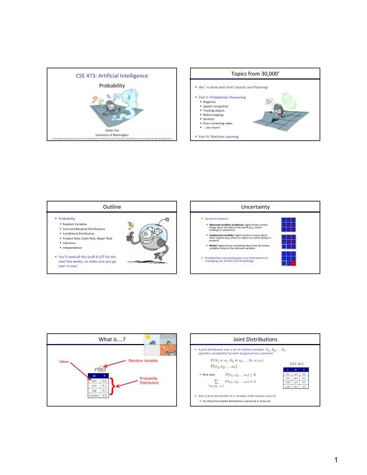
What is….?

W P sun 0.6 rain 0.1 fog 0.3 meteor 0.0

? ?

Random Variable

}

?

Value Probability Distribution

Joint Distributions

§ A joint distribution over a set of random variables: specifies a probability for each assignment (or outcome):

§ Must obey:

§ Size of joint distribution if n variables with domain sizes d?

§ For all but the smallest distributions, impractical to write out! T W P hot sun 0.4 hot rain 0.1 cold sun 0.2 cold rain 0.3

2

Probabilistic Models

§ A probabilistic model is a joint distribution

• ver a set of random variables

§ Probabilistic models:

§ (Random) variables with domains § Joint distributions: say whether assignments (called “outcomes”) are likely § Normalized: sum to 1.0 § Ideally: only certain variables directly interact

§ Constraint satisfaction problems:

§ Variables with domains § Constraints: state whether assignments are possible § Ideally: only certain variables directly interact

T W P hot sun 0.4 hot rain 0.1 cold sun 0.2 cold rain 0.3 T W P hot sun T hot rain F cold sun F cold rain T

Distribution over T,W Constraint over T,W

Events

§ An event is a set E of outcomes § From a joint distribution, we can calculate the probability of any event

§ Probability that it’s hot AND sunny? § Probability that it’s hot? § Probability that it’s hot OR sunny?

§ Typically, the events we care about are partial assignments, like P(T=hot)

T W P hot sun 0.4 hot rain 0.1 cold sun 0.2 cold rain 0.3

Quiz: Events

§ P(+x, +y) ? § P(+x) ? § P(-y OR +x) ?

X Y P +x +y 0.2 +x

• y

0.3

• x

+y 0.4

• x
• y

0.1

Marginal Distributions

§ Marginal distributions are sub-tables which eliminate variables § Marginalization (summing out): Combine collapsed rows by adding T W P hot sun 0.4 hot rain 0.1 cold sun 0.2 cold rain 0.3 T P hot 0.5 cold 0.5 W P sun 0.6 rain 0.4

Quiz: Marginal Distributions

X Y P +x +y 0.2 +x

• y

0.3

• x

+y 0.4

• x
• y

0.1 X P +x

• x

Y P +y

• y

Conditional Probabilities

§ A simple relation between joint and marginal probabilities

§ In fact, this is taken as the definition of a conditional probability

T W P hot sun 0.4 hot rain 0.1 cold sun 0.2 cold rain 0.3 P(b) P(a) P(a,b)

3

Quiz: Conditional Probabilities

X Y P +x +y 0.2 +x

• y

0.3

• x

+y 0.4

• x
• y

0.1

§ P(+x | +y) ? § P(-x | +y) ? § P(-y | +x) ?

Conditional Distributions

§ Conditional distributions are probability distributions over some variables given fixed values of others

T W P hot sun 0.4 hot rain 0.1 cold sun 0.2 cold rain 0.3 W P sun 0.8 rain 0.2 W P sun 0.4 rain 0.6

Conditional Distributions Joint Distribution

Conditional Distribs - The Slow Way…

T W P hot sun 0.4 hot rain 0.1 cold sun 0.2 cold rain 0.3 W P sun 0.4 rain 0.6 SELECT the joint probabilities matching the evidence

Normalization Trick

T W P hot sun 0.4 hot rain 0.1 cold sun 0.2 cold rain 0.3 W P sun 0.4 rain 0.6 T W P cold sun 0.2 cold rain 0.3 NORMALIZE the selection (make it sum to one)

Normalization Trick

T W P hot sun 0.4 hot rain 0.1 cold sun 0.2 cold rain 0.3 W P sun 0.4 rain 0.6 T W P cold sun 0.2 cold rain 0.3 SELECT the joint probabilities matching the evidence NORMALIZE the selection (make it sum to one)

§ Why does this work? Sum of selection is P(evidence)! (P(T=c), here)

Quiz: Normalization Trick

X Y P +x +y 0.2 +x

• y

0.3

• x

+y 0.4

• x
• y

0.1 SELECT the joint probabilities matching the evidence NORMALIZE the selection (make it sum to one)

§ P(X | Y=-y) ?

4

§ Dictionary: “To bring or restore to a normal condition “ § Procedure:

§ Step 1: Compute Z = sum over all entries § Step 2: Divide every entry by Z

§ Example 1

To Normalize

All entries sum to ONE

W P sun 0.2 rain 0.3

Z = 0.5

W P sun 0.4 rain 0.6

§ Example 2

T W P hot sun 20 hot rain 5 cold sun 10 cold rain 15 Normalize Z = 50 Normalize T W P hot sun 0.4 hot rain 0.1 cold sun 0.2 cold rain 0.3

Probabilistic Inference

§ Probabilistic inference = “compute a desired probability from other known probabilities (e.g. conditional from joint)” § We generally compute conditional probabilities

§ P(on time | no reported accidents) = 0.90 § These represent the agent’s beliefs given the evidence

§ Probabilities change with new evidence:

§ P(on time | no accidents, 5 a.m.) = 0.95 § P(on time | no accidents, 5 a.m., raining) = 0.80 § Observing new evidence causes beliefs to be updated

Inference by Enumeration

§ General case:

§ Evidence variables: § Query* variable: § Hidden variables: All variables

* Works fine with multiple query variables, too

§ We want: § Step 1: Select the entries consistent with the evidence § Step 2: Sum out H to get joint

• f Query and evidence

§ Step 3: Normalize

× 1 Z

Inference by Enumeration

§ P(W)? § P(W | winter)? § P(W | winter, hot)?

S T W P summe r hot sun 0.30 summe r hot rain 0.05 summe r cold sun 0.10 summe r cold rain 0.05 winter hot sun 0.10 winter hot rain 0.05 winter cold sun 0.15 winter cold rain 0.20

§ Computational problems?

§ Worst-case time complexity O(dn) § Space complexity O(dn) to store the joint distribution

Inference by Enumeration The Product Rule

§ Sometimes have conditional distributions but want the joint

5

The Product Rule

§ Example:

R P sun 0.8 rain 0.2 D W P wet sun 0.1 dry sun 0.9 wet rain 0.7 dry rain 0.3 D W P wet sun 0.08 dry sun 0.72 wet rain 0.14 dry rain 0.06

The Chain Rule

§ More generally, can always write any joint distribution as an incremental product of conditional distributions

Independence

§ Two variables are independent in a joint distribution if:

§ Says the joint distribution factors into a product of two simple ones § Usually variables aren’t independent!

§ Can use independence as a modeling assumption

§ Independence can be a simplifying assumption § Empirical joint distributions: at best “close” to independent § What could we assume for {Weather, Traffic, Cavity}?

§ Independence is like something from CSPs: what?

Example: Independence?

T W P hot sun 0.4 hot rain 0.1 cold sun 0.2 cold rain 0.3 T W P hot sun 0.3 hot rain 0.2 cold sun 0.3 cold rain 0.2 T P hot 0.5 cold 0.5 W P sun 0.6 rain 0.4

P2(T, W) = P(T)P(W)

Example: Independence

§ N fair, independent coin flips:

H 0.5 T 0.5 H 0.5 T 0.5 H 0.5 T 0.5

Conditional Independence

6

Conditional Independence

§ P(Toothache, Cavity, Catch) § If I have a cavity, the probability that the probe catches in it doesn't depend on whether I have a toothache:

§ P(+catch | +toothache, +cavity) = P(+catch | +cavity)

§ The same independence holds if I don’t have a cavity:

§ P(+catch | +toothache, -cavity) = P(+catch| -cavity)

§ Catch is conditionally independent of Toothache given Cavity:

§ P(Catch | Toothache, Cavity) = P(Catch | Cavity)

§ Equivalent statements:

§ P(Toothache | Catch , Cavity) = P(Toothache | Cavity) § P(Toothache, Catch | Cavity) = P(Toothache | Cavity) P(Catch | Cavity) § One can be derived from the other easily

Conditional Independence

§ Unconditional (absolute) independence very rare (why?) § Conditional independence is our most basic and robust form

• f knowledge about uncertain environments.

§ X is conditionally independent of Y given Z if and only if:

• r, equivalently, if and only if

Conditional Independence

§ What about this domain:

§ Traffic § Umbrella § Raining

Conditional Independence

§ What about this domain:

§ Fire § Smoke § Alarm

Bayes Rule Pacman – Sonar (P4)

[Demo: Pacman – Sonar – No Beliefs(L14D1)]

7

Video of Demo Pacman – Sonar (no beliefs) Bayes’ Rule

§ Two ways to factor a joint distribution over two variables: § Dividing, we get: § Why is this at all helpful?

§ Lets us build one conditional from its reverse § Often one conditional is tricky but the other one is simple § Foundation of many systems we’ll see later (e.g. ASR, MT)

§ In the running for most important AI equation!

That’s my rule!

Inference with Bayes’ Rule

§ Example: Diagnostic probability from causal probability: § Example:

§ M: meningitis, S: stiff neck § Note: posterior probability of meningitis still very small § Note: you should still get stiff necks checked out! Why?

Example givens

P(+s| − m) = 0.01

P(+m| + s) = P(+s| + m)P(+m) P(+s) = P(+s| + m)P(+m) P(+s| + m)P(+m) + P(+s| − m)P(−m) = 0.8 × 0.0001 0.8 × 0.0001 + 0.01 × 0.9999

P(+m) = 0.0001 P(+s| + m) = 0.8 P(cause|effect) = P(effect|cause)P(cause) P(effect)

=0.0079

Ghostbusters Sensor Model

40

P(red | 3) P(orange | 3) P(yellow | 3) P(green | 3) 0.05 0.15 0.5 0.3

Real Distance = 3 Values of Pacman’s Sonar Readings

Ghostbusters, Revisited

§ Let’s say we have two distributions:

§ Prior distribution over ghost location: P(G)

§ Let’s say this is uniform

§ Sensor reading model: P(R | G)

§ Given: we know what our sensors do § R = reading color measured at (1,1) § E.g. P(R = yellow | G=(1,1)) = 0.1

§ We can calculate the posterior distribution P(G|r) over ghost locations given a reading using Bayes’ rule:

[Demo: Ghostbuster – with probability (L12D2) ]

Video of Demo Ghostbusters with Probability

8

Probability Recap

§ Conditional probability § Product rule § Chain rule § Bayes rule § X, Y independent if and only if: § X and Y are conditionally independent given Z: if and only if: