Problem Structure Tree-Structured CSPs Tasmania and mainland are - - PDF document

4/12/15 ¡ 1 ¡

Problem Structure

§ Tasmania and mainland are independent subproblems § Identifiable as connected components of constraint graph § Suppose each subproblem has c variables out of n total § Worst-case solution cost is O((n/c)(dc)), linear in n

§ E.g., n = 80, d = 2, c =20 § 280 = 4 billion years at 10 million nodes/sec § (4)(220) = 0.4 seconds at 10 million nodes/sec

Tree-Structured CSPs

§ Choose a variable as root, order variables from root to leaves such that every node's parent precedes it in the ordering § For i = n : 2, apply RemoveInconsistent(Parent(Xi),Xi) § For i = 1 : n, assign Xi consistently with Parent(Xi) § Runtime: O(n d2)

§ Algorithm for tree-structured CSPs:

§ Order: Choose a root variable, order variables so that parents precede children § Remove backward: For i = n : 2, apply RemoveInconsistent(Parent(Xi),Xi) § Assign forward: For i = 1 : n, assign Xi consistently with Parent(Xi)

§ Runtime: O(n d2) (why?)

Tree-Structured CSPs Nearly Tree-Structured CSPs

§ Conditioning: instantiate a variable, prune its neighbors' domains § Cutset conditioning: instantiate (in all ways) a set of variables such that the remaining constraint graph is a tree § Cutset size c gives runtime O( (dc) (n-c) d2 ), very fast for small c

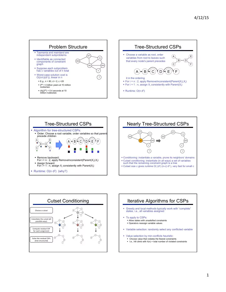
Cutset Conditioning

SA ¡ SA ¡ SA ¡ SA ¡

Instan.ate ¡the ¡cutset ¡(all ¡ possible ¡ways) ¡ Compute ¡residual ¡CSP ¡ for ¡each ¡assignment ¡ Solve ¡the ¡residual ¡CSPs ¡ (tree ¡structured) ¡ Choose ¡a ¡cutset ¡

Iterative Algorithms for CSPs

§ Greedy and local methods typically work with “complete” states, i.e., all variables assigned § To apply to CSPs:

§ Allow states with unsatisfied constraints § Operators reassign variable values

§ Variable selection: randomly select any conflicted variable § Value selection by min-conflicts heuristic:

§ Choose value that violates the fewest constraints § I.e., hill climb with h(n) = total number of violated constraints

4/12/15 ¡ 2 ¡

Example: 4-Queens

§ States: 4 queens in 4 columns (44 = 256 states) § Operators: move queen in column § Goal test: no attacks § Evaluation: h(n) = number of attacks

Performance of Min-Conflicts

§ Given random initial state, can solve n-queens in almost constant time for arbitrary n with high probability (e.g., n = 10,000,000) § The same appears to be true for any randomly-generated CSP except in a narrow range of the ratio

Summary

§ CSPs are a special kind of search problem:

§ States defined by values of a fixed set of variables § Goal test defined by constraints on variable values

§ Backtracking = depth-first search with one legal variable assigned per node § Variable ordering and value selection heuristics help significantly § Forward checking prevents assignments that guarantee later failure § Constraint propagation (e.g., arc consistency) does additional work to constrain values and detect inconsistencies § The constraint graph representation allows analysis of problem structure § Tree-structured CSPs can be solved in linear time § Iterative min-conflicts is usually effective in practice

Local Search Local Search

§ Tree search keeps unexplored alternatives on the fringe (ensures completeness) § Local search: improve a single option until you can’t make it better (no fringe!) § New successor function: local changes § Generally much faster and more memory efficient (but incomplete and suboptimal)

Hill Climbing

§ Simple, general idea:

§ Start wherever § Repeat: move to the best neighboring state § If no neighbors better than current, quit

§ What’s bad about this approach?

§ Complete? § Optimal?

§ What’s good about it?

4/12/15 ¡ 3 ¡

Hill Climbing Diagram Hill Climbing

Star.ng ¡from ¡X, ¡where ¡do ¡you ¡end ¡up ¡? ¡ ¡ ¡ Star.ng ¡from ¡Y, ¡where ¡do ¡you ¡end ¡up ¡? ¡ ¡ Star.ng ¡from ¡Z, ¡where ¡do ¡you ¡end ¡up ¡? ¡

Simulated Annealing

§ Idea: Escape local maxima by allowing downhill moves

§ But make them rarer as time goes on

55

Simulated Annealing

§ Theoretical guarantee:

§ Stationary distribution: § If T decreased slowly enough, will converge to optimal state!

§ Is this an interesting guarantee? § Sounds like magic, but reality is reality:

§ The more downhill steps you need to escape a local

• ptimum, the less likely you are to ever make them all

in a row § People think hard about ridge operators which let you jump around the space in better ways

Genetic Algorithms

§ Genetic algorithms use a natural selection metaphor

§ Keep best N hypotheses at each step (selection) based on a fitness function § Also have pairwise crossover operators, with optional mutation to give variety

§ Possibly the most misunderstood, misapplied (and even maligned) technique around

Example: N-Queens

§ Why does crossover make sense here? § When wouldn’t it make sense? § What would mutation be? § What would a good fitness function be?

4/12/15 ¡ 4 ¡

GA’s for Locomotion

Hod Lipson’s Creative Machines Lab @ Cornell