Program Analysis discrete math refresher READING: Textbook - - PowerPoint PPT Presentation

csci 210: Data Structures

Program Analysis

1

Summary

• Summary
• analysis of algorithms
• asymptotic analysis
• big-O
• big-Omega
• big-theta
• asymptotic notation
• commonly used functions
• discrete math refresher
• READING:
• Textbook chapter 2 (p. 13-26)

Analysis of algorithms

• Analysis of algorithms and data structure is the major force that drives the design of

solutions.

• there are many solutions to a problem: pick the one that is the most efficient
• how to compare various algorithms? Analyze algorithms.
• Algorithm analysis: analyze the cost of the algorithm
• cost = time: How much time does this algorithm require?
• The primary efficiency measure for an algorithm is time
• all concepts that we discuss for time analysis apply also to space analysis
• cost = space: How much space (i.e. memory) does this algorithm require?
• cost = space + time
• etc
• Running time of an algorithm
• increases with input size
• n inputs of same size, can vary from input to input
• e.g.: linear search an un-ordered array
• depends on hardware
• CPU speed, hard-disk, caches, bus, etc
• depends on OS, language, compiler, etc
• Everything else being equal
• we’d like to compare algorithms
• we’d like to study the relationship running time vs. size of input
• How to measure running time of an algorithm?
• 1. experimental studies
• 2. theoretical analysis
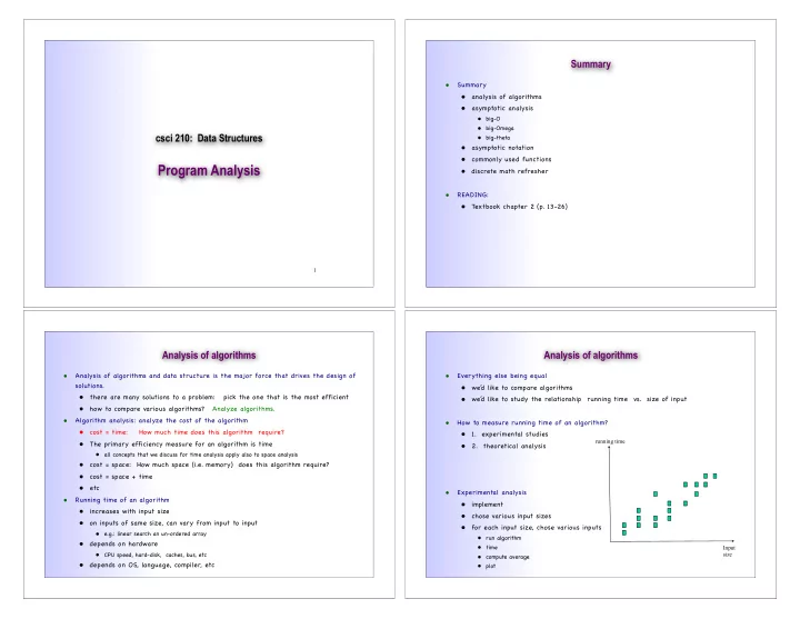
• Experimental analysis
• implement
• chose various input sizes
• for each input size, chose various inputs
• run algorithm
• time
• compute average
• plot

Analysis of algorithms

Input size running time

Experimental analysis

• Limitations
• need to implement the algorithm
• need to implement all algorithms that we want to compare
• need many experiments
• try several platforms
• Advantages
• find the best algorithm in practice
• We would like to analyze algorithms without having to implement them
• Basically, we would like to be able to look at two algorithms flowcharts and decide

which one is better

Input size running time

Theoretical analysis

• RAM model of computation
• Assume all operations cost the same
• Assume all data fits in memory
• Running time (efficiency) of an algorithm:
• the number if operations executed by the algorithm
• Does this reflect actual running time?
• multiply nb. of instructions by processor speed
• 1GHz processor ==> 10^9 instructions/second
• Is this accurate?
• Not all instructions take the same...
• Various other effects.
• Overall, it is a very good predictor of running time in most cases.

Terminology

• Notation: n = size of the input to the problem
• Running time:
• number of operations/instructions executed on an input of size n
• expressed as function of n: f(n)
• For an input of size n, running time may be smaller on some inputs than on others
• Best case running time:
• the smallest number of operations on an input of size n
• Worst-case running time:
• the largest number of operations on an input of size n
• For any n
• best-case running time(n) <= running time(n) <= worst-case running time (n)
• Ideally, want to compute average-case running time
• need to know the distribution of the input
• ften assume uniform distribution (all inputs are equally likely), but this may not

be realistic

Running time

• Expressed as functions of n: f(n)
• The most common functions for running times are the following:
• constant time :
• f(n) = c
• logarithmic time
• f(n) = lg n
• linear time
• f(n) = n
• n lg n
• f(n) = n lg n
• quadratic
• f(n) = n2
• cubic
• f(n) = n3
• exponential
• f(n) = an

Constant running time

• f(n) = c
• Meaning: for any n, f(n) is a constant c
• Elementary operations
• arithmetic operations
• boolean operations
• assignment statement
• function call
• access to an array element a[i]
• etc

Logarithmic running time

• f(n) = lg c n
• Logarithm definition:
• x = log c n if and only of c x = n
• by definition, log c 1 = 0
• In algorithm analysis we use the ceiling to round up to an integer
• the ceiling of x: the smallest integer >= x
• e.g. ceil(log b n) is the number of times you can divide n by b until you get a

number <= 1

• e.g.
• ceil(log 2 8) = 3
• ceil(log 2 10) = 4
• Notation: lg n = log 2 n
• Refresher: Logarithm rules
• Note: computing lg n on your calculator
• lg n = log 10 n / log 10 2

Exercises

Simplify these expressions

• lg 2n =
• lg (n/2) =
• lg n3 =
• lg 2n
• log 4 n =
• 2 lg n

Binary search

//return the index where key is found in a, or -1 if not found public static int binarySearch(int[] a, int key) {

int left = 0; int right = a.length-1; while (left <= right) {

int mid = left + (right-left)/2; if (key < a[mid]) right = mid-1; else if (key > a[mid]) left = mid+1; else return mid;

}

//not found return -1; }

• running time:
• best case: constant
• worst-case: lg n

Why? input size halves at every iteration of the loop

Linear running time

• f(n) = n
• Example:
• doing one pass through an array of n elements
• e.g.
• finding min/max/average in an array
• computing sum in an array
• search an unordered array (worst-case)

int sum = 0 for (int i=0; i< a.length; i++) sum += a[i]

n-lg-n running time

• f(n) = n lg n
• grows faster than n (i.e. it is slower than n)
• grows slower than n2
• Examples
• performing n binary searches in an ordered array
• sorting

Quadratic time

• f(n) = n2
• appears in nested loops
• enumerating all pairs of n elements
• Example 1:

for (i=0; i<n; i++) for (j=0; j<n; j++) //do something

• Example2:

//selection sort: for (i=0; i<n-1; i++) minIndex = index-of-smallest element in a[i..n-1] swap a[i] with a[minIndex]

• running time:
• index-of-smallest element in a[i..j] takes j-i+1 operations
• n + (n-1) + (n-2) + (n-3) + ... + 3 + 2 + 1
• this is n2

Math refresher

• Lemma:
• 1+ 2 + 3 + 4 + ..... + (n-2) + (n-1) + n = n(n+1)/2 (arithmetic sum)
• Proof:

Cubic running times

• Cubic running time: f(n) = n3
• Examples:
• nested loops
• Enumerate all triples of elements
• Imagine cities on a map. Are there 3 cities that no two are not joined by a

road?

• Solution: enumerate all subsets of 3 cities. There are n chose 3 different subsets, which is
• rder n3.
• In general, a polynomial running time: f(n) = nd, d>0

Exponential running time

• Exponential running time: f(n) = an , a > 1
• Examples:
• running time of Tower of Hanoi (see later)
• moving n disks from A to B requires at least 2n moves; which means it requires at least this

much time

• Math refresher: exponent rules

Asymptotic analysis

• Focus on the growth of rate of the running time, as a function of n
• That is, ignore the constant factors and the lower-order terms
• Focus on the big-picture
• Example: we’ll say that 2n, 3n, 5n, 100n, 3n+10, n + lg n, are all linear
• Why?
• constants are not accurate anyways
• perations are not equal
• capture the dominant part of the running time
• Notations:
• Big-Oh:
• express upper-bounds
• Big-Omega:
• express lower-bounds
• Big-Theta:
• express tight bounds (upper and lower bounds)

Big-Oh

• Definition: f(n) is O(g(n)) if exists c >0 such that f(n) <= cg(n) for all n >= n0
• Intuition:
• big-oh represents an upper bound
• when we say f is O(g) this means that
• f <= g asymptotically
• g is an upper bound for f
• f stays below g as n goes to infinity
• Examples:
• 2n is O(n)
• 100n is O(n)
• 10n + 50 is O(n)
• 3n + lg n is O(n)
• lg n is O(log_10 n)
• lg_10 n is O(lg n)
• 5n4 + 3n3 + 2n2 + 7n + 100 is O(n4)

Big-Oh

• 2n2 + n lg n +n + 10
• is O(n2 + n lg n)
• is O(n3)
• is O(n4)
• isO(n2)
• 3n + 5
• is O(n10)
• is O(n2)
• is O(n+lg n)
• Let’

s say you are 2 minutes away from the top and you don’t know that. You ask: How much further to the top?

• Answer 1: at most 3 hours (True, but not that helpful)
• Answer 2: just a few minutes.
• When finding an upper bound, the goal is to find the best one possible.

Exercises

• Using the definition, show the following:
• 100n is O(n)
• n is O(100n)
• 15n+7 is O(n)
• 15n+7 is O(n2)
• 5n+4 is O(2n+3)
• 4n2+9n+8 is O(n2)

22

Exercises

Write Big-Oh upper bounds for each of the following.

• 10n - 2
• 5n3 + 2n2 +10n +100
• 5n2 + 3nlg n + 2n + 5
• 20n3 + 10n lg n + 5
• 3 n lgn + 2
• 2n+2 + n3 + 20
• 2n + 100 lg n

Big-Omega

• Definition:
• f(n) is Omega(g(n)) if exists c>0 such that f(n) >= cg(n) for all n >= n0
• Intuition:
• big-omega represents a lower bound
• when we say f is Omega(g) this means that
• f >= g asymptotically
• g is a lower bound for f
• f stays above g as n goes to infinity
• Examples:
• 3nlgn + 2n is Omega(n lg n)
• 2n + 3 is Omega(n)
• 4n2 +3n + 5 is Omega(n)
• 4n2 +3n + 5 is Omega(n2)
• O() and Omega() are symmetrical:
• f(n) is g(n) <====> g(n) is Omega(f(n))

Big-Theta

• Definition:
• f(n) is Theta(g(n)) if f(n) is O(g(n)) and f is Omega(g(n))
• i.e. there are constants c’ and c’’ such that c’g(n) <= f(n) <= c”g(n)
• Intuition:
• f and g grow at the same rate, up to constant factors
• Theta captures the order of growth
• Examples:
• 3n + lg n + 10 is O(n) and Omega(n) ==> is Theta(n)
• 2n2 + n lg n + 5 is Theta(n2)
• 3lgn +2 is Theta(lgn)

Asymptotic Analysis

• Find tight bounds for the best-case and worst-case running times
• Running time is Omega(best-case running time)
• Running time is O(worst-case running time)
• Example:
• binary search is Theta(1) in the best case
• binary search is Theta(lg n) in the worst case
• binary search is Omega(1) and O(lg n)
• Usually we are interested the worst-case running time
• a Theta-bound for the worst-case running time
• Example:
• worst-case binary search is Theta(lg n)
• worst-case linear search is Theta(n)
• worst-case insertion sort is Theta(n^2)
• worst-case bubble-sort is O(n^2)
• worst-case find-min in an array is Theta(n)
• It is correct to say worst-case binary search is O(lg n), but a Theta-bound is better

Asymptotic Analysis

• Suppose we have two algorithms for a problem:
• Algorithm A has a running time of O(n)
• Algorithm B has a running time of O(n2)
• Which is better?
• Suppose we have two algorithms for a problem:
• Algorithm A has a running time of Theta(n)
• Algorithm B has a running time of Theta(n2)
• Which is better?
• rder classes of functions by their oder of growth
• Theta(1) < Theta(lg n) < Theta(n) < Theta(nlgn) < Theta(n2) < Theta(n3) < Theta(2n)
• Theta(n) is better than Theta(n2), etc
• Cannot distinguish between algorithms in the same class
• two algorithms that are Theta(n) worst-case are equivalent theoretically
• optimization of constants can be done at implementation-time

Asymptotic Analysis

Order of growth matters

• Example:
• Say n = 109 (1 billion elements)
• 10 MHz computer ==> 1 instruction takes 10-7 seconds
• Binary search would take
• Theta(lg n) = lg 109 x 10-7 sec = 30 x 10-7 sec = 3 microsec
• Sequential search would take
• Theta(n)= 109 x 10-7 sec = 100 seconds
• Finding all pairs of elements would take
• Theta(n2) = (109)2 x 10-7 sec = 1011 seconds = 3170 years
• Imagine Theta(n3)
• Imagine Theta(2n)

Order of growth matters

n lg n n n lg n n^2 n^3 2^n 8 3 8 24 64 512 256 16 4 16 64 256 4,096 65,536 32 5 32 160 1,024 32,768

4,294,967,296

64 6 64 384 4,096 262,144

1.8 x 10^19

128 7 128 896 16,384 2,097,152

3.40 x 10^38

256 8 256 2.048 65,536

16,777,216

1.15 x 10^77

512 9 512 4,608 262,144

134,217,728

1.34 x 10^154

1024 10 1024 10242 20 1,048,576 109

• Assume we have a 1 GHz computer.
• This means an instruction takes 1 microsecond (10-9 seconds).
• We have 3 algorithms:
• A: 400n
• B 2n2
• C: 2n
• What is the maximum input size that can be solved with each algorithm in:
• 1 second
• 1 minute
• 1 hour

Running time (in microseconds)

1 sec 1 min 1 hour 400n 2n2 2n

Exercise

• We have an array X containing a sequence of numbers. We want to compute another

array A such that A[i] represents the average X[0] + X[1] + ... X[i]/ (i+1).

• A[0] = X[0]
• A[1] = (X[0] + X[1])/ 2
• A[2] = (X[0] + X[1] + X[2]) / 3
• ...
• The first i values of X are referred to as the i-prefix of X.

X[0] + ... X[i] is called prefix-sum, and A[i] prefix average.

• Application: In Economics. Imagine that X[i] represents the return of a mutual fund

in year i. A[i] represents the average return over i years.

• Write a function that creates, computes and returns the prefix averages.

double[] computePrefixAverage(double[] X)

• Analyze your algorithm (worst-case running time).

Asymptotic Analysis: Overview

• Running time = number of instructions
• RAM model of computation
• Want the worst-case running time as a function of input size
• Find the tight order of growth of the worst-case running time
• a Theta-bound
• Classification of growth rates

Theta(1) < Theta(lg n) < Theta(n) < Theta(nlgn) < Theta(n2) < Theta(n3) < Theta(2n)

• At the algorithm design level, we want to find the most efficient algorithm in terms of

growth rate

• We can optimize constants at the implementation step