Q. Why do we have a brain? A. To produce adaptable and complex - - PowerPoint PPT Presentation

Probabilistic mechanisms in human sensorimotor control

Daniel Wolpert, University College London

• movement is the only way we have of

– Interacting with the world – Communication: speech, gestures, writing

• sensory, memory and cognitive processes future motor outputs
• Q. Why do we have a brain?

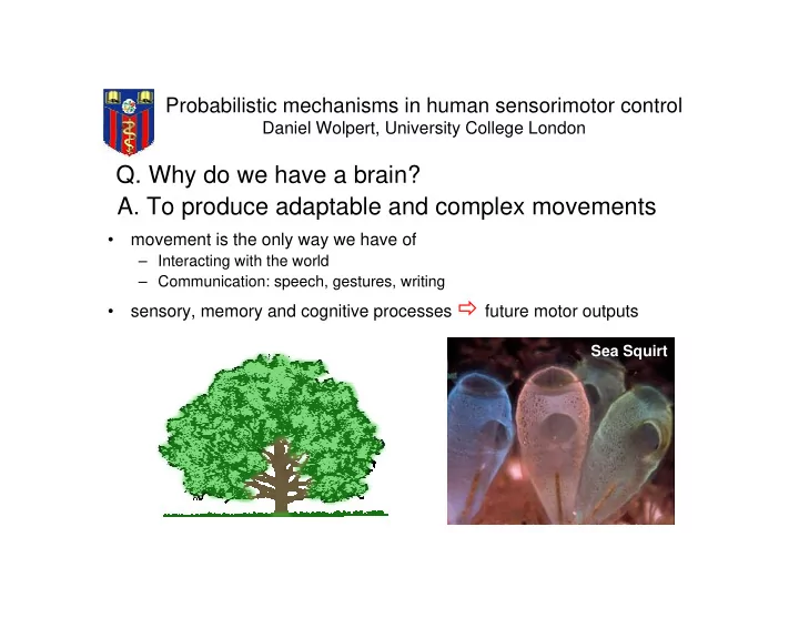
Sea Squirt

• A. To produce adaptable and complex movements

1000 1500 2000 2500 3000 3500

Why study computational sensorimotor control? Year Pages

r2=0.96

1980 1990 2000 2010 2020 2030 2040 2050 500

Experiments Theory

Principles of Neural Science, Kandel et al.

vs. What to move where vs. Moving

The complexity of motor control

Noise makes motor control hard

Noise = randomness The motor system is Noisy Perceptual noise

– Limits resolution

Motor Noise

– Limits control

Noisy Partial Noisy

Ambiguous Variable

David Marr’s levels of understanding (1982)

1) the level of computational theory

• f the system

2) the level of algorithm and representation, which are used make computations 3) the level of implementation: the underlying hardware or "machinery" on which the computations are carried out.

Tutorial Outline

– Sensorimotor integration

• Static multi-sensory integration
• Bayesian integration
• Dynamic sensor fusion & the Kalman filter

– Action evaluation

• Intrinsic loss function
• Extrinsic loss functions

– Prediction

• Internal model and likelihood estimation
• Sensory filtering

– Control

• Optimal feed forward control
• Optimal feedback control

– Motor learning of predictable and stochastic environments

Review papers on www.wolpertlab.com

Multi-sensory integration

Multiple modalities can provide information about the same quantity

• e.g. location of hand in space

– Vision – Proprioception

• Sensory input can be

– Ambiguous – Noisy

• What are the computations used in

integrating these sources?

Ideal Observers

Maximum likelihood estimation (MLE)

i i

x x ε = +

1 2

( , ..., | )

n

P x x x x

1

( | )

n i i

P x x

=

=∏

2

(0, )

i i

N ε σ =

( )

2 2 1 1

ˆ with

n i i i i n i j j

x w x w σ σ

− − = =

= =

∑ ∑

( )

1 2 2 2 ˆ 1 n x i k j

k σ σ σ

− − =

= < ∀

∑

2

x

1

x x Consider signals , {1 }

i

n x i n = …

Two examples of multi-sensory integration

Visual-haptic integration (Ernst & Banks 2002)

Two alternative force choice size judgment

• Visual
• Haptic
• Visual-haptic (with discrepancy)

Visual-haptic integration

Measure

• Visual reliability
• Haptic reliability
• Predict
• Visual + Haptic noise
• Weighting of

2 V

σ

2 H

σ

2

H

σ

Probability

Size

Probability Size difference

2

H

σ

H

σ

H

σ

Visual-haptic integration

( )

2 2 1 2 2 2

1

i i n j j V H V H V H

w w w w σ σ σ σ σ

− − =

= = = − +

∑

( )

2 2 1 2 2 ˆ 2 2 1 n V H x i j V H

σ σ σ σ σ σ

− − =

= = +

∑

Weights Standard deviation (~threshold) Optimal integration of vision and haptic information in size judgement

Visual-proprioceptive integration

Classical claim from prism adaptation “vision dominates proprioception”

Reliability of proprioception depends on location

(Van Beers, 1998)

Reliability of visual localization is anisotropic

Integration models with discrepancy

Winner takes all Linear weighting of mean Optimal integration

ˆ (1 )

V H

w w = + − x x x ˆ

V H

A B = + x x x

1 1 1 1 1

( ) ( )

PV P V PV PV P P V V

µ µ µ

− − − − −

Σ = Σ + Σ = Σ Σ + Σ

Prisms displace along the azimuth

• Measure V and P
• Apply visuomotor discrepancy during right hand reach
• Measure change in V and P to get relative adaptation

Vision 0.33 Prop 0.67

(Van Beers, Wolpert & Haggard, 2002)

Visual-proprioceptive discrepancy in depth

Adaptation Vision 0.72 Prop 0.28

Visual adaptation in depth > visual adaptation in azimuth (p<0.01) > Proprioceptive adaptation in depth (p<0.05) Proprioception dominates vision in depth

Priors and Reverend Thomas Bayes

“I now send you an essay which I have found among the papers of our deceased friend Mr Bayes, and which, in my opinion, has great merit....” Essay towards solving a problem in the doctrine of chances. Philosophical Transactions of the Royal Society of London, 1764.

1702-1761

Bayes rule

• A and B

( , ) P A B =

( | ) P A B

( | ) ( ) P B A P A =

Belief instate sensory inpu AFTER t

• Posterior

( ) P B

P(state|sensoryinput)

Prior BEFORE Belief in state sensory input

• Neuroscience

A= State of the world B=Sensory Input A = Disease B = Positive blood test

Likelihood Evidence

• P(sensoryinput|state)P(state)

= P(sensoryinput)

• AgivenB

Bayesian Motor Learning

=

Optimal estimate (Posterior) Bayes rule

+

Task statistics (Prior) Not all locations are equally likely Sensory feedback (Evidence) Combine multiple cues to reduce uncertainty

Estimate

Evidence Prior

P (sensor P(state| yinput|s sensory tate P input) (st ) ) ate ∝

Real world tasks have variability, e.g. estimating ball’s bounce location

Does sensorimotor learning use Bayes rule? If so, is it implemented

• Implicitly: mapping sensory inputs to motor outputs to minimize error?
• Explicitly: using separate representations of the statistics of the prior and sensory noise?

(Körding & Wolpert, Nature, 2004)

Prior

Lateral shift (cm) Probability

0 1 2

Task in which we control 1) prior statistics of the task 2) sensory uncertainty

(Körding & Wolpert, Nature, 2004)

Prior

Lateral shift (cm) Probability

0 1 2

Task in which we control 1) prior statistics of the task 2) sensory uncertainty

Sensory Feedback

Likelihood

Generalization Learning

After 1000 trials

2 cm shift

1cm No visual feedback

Probability 0 1 2

Lateral shift (cm)

0 1 2

Bayesian Compensation

Lateral shift (cm)

Models

Full Compensation

Lateral shift (cm)

0 1 2

0 1 2 Lateral Shift (cm) Average Error Bias (cm)

1

• 1

0 1 2 Lateral Shift (cm) Average Error Bias (cm)

1

• 1

Mapping

0 1 2 Lateral shift (cm)

0 1 2 Lateral Shift (cm) Average Error Bias (cm)

1

• 1

Supports model 2: Bayesian

Results: single subject

Full Bayes Map

0 1 2 Lateral Shift (cm) Average Error Bias (cm)

Supports model 2: Bayesian

Results: 10 subjects

Full Bayes Map

0 1 2 Lateral Shift (cm) Average Error Bias (cm)

• 0.5

1 2.5 1

lateral shift [cm]

Lateral shift (cm) Inferred Prior (normalized)

Bayesian integration

Subjects can learn

• multimodal priors
• priors over forces
• different priors one after the other

(Körding& Wolpert NIPS 2004, Körding, Ku & Wolpert J. Neurophysiol. 2004)

Statistics of the world shape our brain Objects Configurations of our body

• Statistics of visual/auditory stimuli representation visual/auditory cortex
• Statistics of early experience what can be perceived in later life

(e.g. statistics of spoken language)

Statistics of action

• 4 x 6-DOF electromagnetic sensors
• battery & notebook PC

With limited neural resources statistics of motor tasks motor performance

Phase relationships and symmetry bias

Multi-sensory integration

• CNS

– In general the relative weightings of the senses is sensitive to their direction dependent variability – Represents the distribution of tasks – Estimates its own sensory uncertainty – Combines these two sources in a Bayesian way

• Supports an optimal integration model

Loss Functions in Sensorimotor system

What is the performance criteria (loss, cost, utility, reward)?

• Often assumed in statistics & machine learning

– that we wish to minimize squared error for analytic or algorithmic tractability

• What measure of error does the brain care about?

Target Position Posterior Probability

Prior Like Posterior lihood

P(sensoryi P(state|sensoryinpu nput|state)P(state t) ) ∝

• [

] ( , ) ( | _ ) _ ˆ ( ) arg min [ ]

B actions

E Loss Loss state action P state sensory input dsensory input Bayesestimator x s E Loss = =

∫

Loss function

3 1 2 2

Target

Scenario 1 Scenario 2

( ) f error

2

Loss error =

1 2

Loss error = Loss error =

Loss=4+4=8 Loss=1+9=10 Loss=2+2=4 Loss=1+3=4 Loss=1+1.7=2.7 Loss=1.4+1.4=2.8

Virtual pea shooter

Mean Starting location

Position (cm) Probability

• 0.2 0 0.2

(Körding & Wolpert, PNAS, 2004)

Probed distributions and optimal means

Possible Loss functions

2

Loss ( ) error =

MEAN

• 2 -1 0 1 2

Error (cm) ρ=0.2 ρ=0.3 ρ=0.5 ρ=0.8

Distributions

MODE Maximize Hits

• 2 -1 0 1 2

Error (cm)

MEDIAN

Loss error =

Robust estimator

Shift of mean against asymmetry (n=8)

Mean squared error with robustness to outliers

0.1 1.0 1.3 1.5 1.7 1.9 2.1 2.3 2.5 2.7 2.9 3.1 3.3 3.5 3.7 3.9

α=

Loss

i

errorα = ∑ Personalised loss function

Bayesian decision theory

Increasing probability of avoiding keeper Increasing probability of being within the net

Imposed loss function (Trommershäuser et al 2003)

• 100
• 500

+100 +100 +100

Optimal performance with complex regions

State estimation

• State of the body/world

– Set of time-varying parameters which together with

• Dynamic equations of motion
• Fixed parameters of the system (e.g. mass)

– Allow prediction of the future behaviour

• Tennis ball

– Position – Velocity – Spin

State estimation

NOISE NOISE

Observer

Kalman filter

• Minimum variance estimator

– Estimate time-varying state – Can’t directly observe state but only measurement

1 t t t t

A B

+ =

+ + x x u w

1 t t t

C

+ =

+ y x v

1

ˆ ˆ ˆ [ ]

t t t t t t

A B K C

+ =

+ + − x x u y x

State estimation

1 ForwardDynamicModel

ˆ ˆ ˆ [ ]

t t t t t t

A B K C

+ =

+ + − x x u y x

Kalman Filter

• Optimal state estimation is a mixture

– Predictive estimation (FF) – Sensory feedback (FB)

Eye position

Location of object based on retinal location and gaze direction Percept Actual

Motor command FM Eye Position

Sensory likelihood

(Wolpert & Kawato, Neural Networks 1998 Haruno, Wolpert, Kawato, Neural Computation 2001)

P(sensor P(state| yinput|s sensory tate input) P(st ) ) ate ∝

Sensory prediction

Our sensors report

• Afferent information:

changes in outside world

• Re-afferent information:

changes we cause

+ = Internal source External source

Tickling

Self-administered tactile stimuli rated as less ticklish than externally administered tactile stimuli. (Weiskrantz et al, 1971)

Does prediction underlie tactile cancellation in tickle?

0.5 1 1.5 2 2.5 3 Self-produced tactile stimuli Robot-produced tactile stimuli Condition Tickle rating rank

Gain control or precise spatio-temporal prediction?

P<0.001

Spatio-temporal prediction

0.5 1 1.5 2 2.5 3 3.5 4 Delay 0ms Delay 100ms Delay 200ms Delay 300ms Robot- produced tactile stimuli Condition Tickle rating rank

P<0.001 P<0.001

0.5 1 1.5 2 2.5 3 3.5 4 0 degrees 30 degrees 60 degrees 90 degrees External

Condition Tickle rating rank P<0.001 P<0.001

(Blakemore, Frith & Wolpert. J. Cog. Neurosci. 1999)

The escalation of force

Tit-for-tat

Force escalates under rules designed to achieve parity: Increase by ~40% per turn

(Shergill, Bays, Frith & Wolpert, Science, 2003)

Perception of force

70% overestimate in force

Perception of force

Labeling of movements

Large sensory discrepancy

Defective prediction in patients with schizophrenic

• The CNS predicts sensory

consequences

• Sensory cancellation in

Force production

• Defects may be related to

delusions of control

Patients Controls

Motor Learning

Required if:

• organisms environment, body or task change
• changes are unpredictable so cannot be pre-specified
• want to master social convention skills e.g writing

Trade off between:

– innate behaviour (evolution)

• hard wired
• fast
• resistant to change

– learning (intra-life)

• adaptable
• slow
• Maleable

Motor Learning

Actual behaviour

Predicted outcome can be compared to actual

• utcome to generate an

error

Supervised learning is good for forward models

Weakly electric fish (Bell 2001)

Produce electric pulses to

• recognize objects in the dark or in murky habitats
• for social communication.

The fish electric organ is composed of electrocytes,

• modified muscle cells producing action potentials
• EOD = electric organ discharges
• Amplitude of the signal is between 30 mV and 7V
• Driven by a pacemaker in medulla, which triggers each discharge

Sensory filtering

Skin receptors are derived from the lateral line system

Removal of expected or predicted sensory input is one of the very general functions of sensory processing. Predictive/associative mechanisms for changing environments

Primary afferent terminate in cerebellar-like structures

Primary afferents terminate on principal cells either directly or via interneurons

Block EOD discharge with curare

Specific for Timing (120ms), Polarity, Amplitude & Spatial distribution

Proprioceptive Prediction

Tail bend affects feedback Passive Bend phase locked to stimulus:

Bend

Learning rule

Changes in synaptic strength requires principal cell spike discharge Change depends on timing of EPSP to spike Anti-Hebbian learning T1 T2 T2-T1

• Forward Model can be learned through self-supervised learning
• Anti-hebbian rule in Cerebellar like structure of he electric fish

Motor planning (what is the goal of motor control)

Duration Hand Trajectory Joint Muscles

• Tasks are usually specified at a symbolic level
• Motor system works at a detailed level, specifying muscle activations
• Gap between high and low-level specification
• Any high level task can be achieved in infinitely many low-level ways

Eye-saccades Arm- movements

Motor evolution/learning results in stereotypy

Stereotypy between repetitions and individuals

Time (ms)

• Main sequence
• Donder’s law
• Listings Law
• 2/3 power law
• Fitts’ law

Models

HOW models

– Neurophysiological or black box models – Explain roles of brain areas/processing units in generating behavior

WHY models

– Why did the How system get to be the way it is? – Unifying principles of movement production

• Evolutionary/Learning

– Assume few neural constraints

The Assumption of Optimality

Movements have evolved to maximize fitness

– improve through evolution/learning – every possible movement which can achieve a task has a cost – we select movement with the lowest cost

Overall cost = cost1 + cost2 + cost3 ….

Optimality principles

• Parsimonious performance criteria

Elaborate predictions

• Requires

– Admissible control laws – Musculoskeletal & world model – Scalar quantitative definition of task performance – usually time integral of f(state, action)

Open-loop

• What is the cost

– Occasionally task specifies cost

• Jump as high as possible
• Exert maximal force

– Usually task does not specify the cost directly

• Locomotion well modelled by energy minimization
• Energy alone is not good for eyes or arms

What is the cost?

Saccadic eye movements

• little vision over 4 deg/sec
• frequent 2-3 /sec
• deprives us of vision for 90

minutes/day ⇒Minimize time

Arm movements

Movements are smooth – Minimum jerk (rate of change of acceleration) of the hand (Flash & Hogan 1985)

2 2 4 5 3 4 5 3

( ) ( ) ( ) ( )(15 6 10 ) ( ) ( )(15 6 10 ) /

T T T

Cost x t y t dt x t x x x y t y y y t T τ τ τ τ τ τ τ = + = + − − − = + − − − =

∫

Smoothness

• Minimum Torque change (Uno et al, 1989)

Shoulder torque Elbow torque

2 2

( ) ( )

T s e

Cost t t dt τ τ = +

∫

The ideal cost for goal-directed movement

• Makes sense - some evolutionary/learning advantage
• Simple for CNS to measure
• Generalizes to different systems

– e.g. eye, head, arm

• Generalizes to different tasks

– e.g. pointing, grasping, drawing

→ Reproduces & predicts behavior

Motor command noise

Motor System Noise Position Error minimized by rapidity

Fundamental constraint=Signal-dependent noise

• Signal-dependent noise:

– Constant coefficient of variation – SD (motor command) ~ Mean (motor command)

• Evidence from

– Experiments: SD (Force) ~ Mean (Force) – Modelling

• Spikes drawn from a renewal process
• Recruitment properties of motor units

(Jones, Hamilton & Wolpert , J. Neurophysiol., 2002)

Task optimization in the presence of SDN

Given SDN, Task Given SDN, Task ≡ ≡ optimizing

• ptimizing f(statistics

f(statistics) )

An average motor command ⇒ probability distribution (statistics) of movement.

Controlling the statistics of action Controlling the statistics of action

Finding optimal trajectories for linear systems

2 2 2

( ) ( )

u t

k u t σ =

time

T M

x(t)

[ ( )] ( ) ( )

M

E x M u p M d A τ τ τ = − =

∫

2 2 2 2 2

[ ( )] [ ( ) ( )] [ ( )] ( ) ( ) ( ) ( ) ( )

M M M M

Var x T Var u p T d Var u p T d k u p T d w u d τ τ τ τ τ τ τ τ τ τ τ τ = − = − = − =

∫ ∫ ∫ ∫

time p(t) Impulse response Signal-dependent noise

( ) ( )

[ ( )] ( ) ( )

M n n

E x M u p M d τ τ τ = − =

∫

Cost Constraints System A Linear constraints with quadratic cost: can use quadratic programming or isoperimetric optimization

Saccade predictions

SDN

Motor command Jerk 3rd order linear system

100 200 20 Time (ms) Degrees

Prediction: very slow saccade

22 degree saccade in 270 ms (normally ~ 70 ms)

Head free saccade

100 200 300 400 500 600 700 800 20 40 60 80 100 120

Degrees Time (ms)

Head Gaze Eye

Τ1=0.3 Τ2=0.3 Τ1=0.15 Τ2=0.08

Free parameter, eye:head noise

100 200 300 400 500 600 700 800 20 40 60 80 100 120

Time (ms) Degrees

Eye Head Gaze

(Tomlinson & Bahra, 1986)

Coordination: Head and eye

For a fixed duration (T), Var(A)=k A2

Var(A)=k A2 Var(A)= k (A/2)2 + k (A/2)2

= k A2 /2

Var(A)=k A2

Eye only Head only Eye & Head

Movement extent vs. target eccentricity

Gaze amplitude

Angular deviation at acquisition

Eye Head

Gaze amplitude

20 40 60 80 100 120 140 10 20 30 40 50 60 70 80 90 100

} }

Head Eye

Arm movements

Drawing (⅔ power law) f=path error Obstacle avoidance f= limit probability of collision Smoothness Non smooth movement ⇒ requires abrupt change in velocity ⇒ given low pass system ⇒ large motor command ⇒ increased noise Smoothness ⇒ accuracy

Feedforward control

• Ignores role of feedback
• Generates desired movements
• Cannot model trial-to-trial variability

Optimal feedback control (Todorov 2004)

– Optimize performance over all possible feedback control laws – Treats feedback law as fully programmable

• command=f(state)
• Models based on reinforcement learning optimal cost-to-go functions
• Requires a Bayesian state estimator

Minimal intervention principle

• Do not correct deviations

from average behaviour unless they affect task performance

– Acting is expensive

• energetically
• noise

– Leads to

• uncontrolled manifold
• synergies

U n c

• n

t r

• l

l e d m a n i f

• l

d

Optimal control with SDN

• Biologically plausible theoretical underpinning

for both eye, head, arm movements

• No need to construct highly derived signals to

estimate the cost of the movement

• Controlling statistics in the presence of noise

What is being adapted?

• Possible to break down the control process:
• Visuomotor rearrangements
• Dynamic perturbations
• [timing, coordination , sequencing]
• Internal models captures the relationship

between sensory and motor variables

Altering dynamics

Altering Kinematics

Representation of transformations

Look-up Table Non-physical Parameters θ=f(x,ω) Physical Parameters θ=acos(x/L)

High storage High flexibility Low Generalization Low storage Low flexibility High Generalization

θ x L

÷

asin

x θ L x θ

x θ 1 10 3 35 . . . .

Generalization paradigm

• Baseline

– Assess performance over domain of interest – (e.g. workspace)

• Exposure

– Perturbation: New task – Limitation: Limit the exposure to a subdomain

• Test

– Re-assess performance

• ver entire domain of

interest

Difficulty of learning

(Cunningham 1989, JEPP-HPP)

• Rotations of the visual field

from 0—180 degrees Difficulty

• increases from 0 to 90
• decreases from 120 to 180
• What is the natural

parameterization

Viscous curl field

(Shadmehr & Mussa-Ivaldi 1994, J. Neurosci.)

Representation from generalization: Dynamic 1. Test: Movements over entire workspace 2. Learning – Right-hand workspace – Viscous field 3. Test: Movements over left workspace Two possible interpretations force = f(hand velocity)

• r torque=f(joint velocity)

Joint-based learning of dynamics

(Shadmehr & Mussa-Ivaldi 1994, J. Neurosci.)

Left hand workspace Before After with Cartesian field

Visuomotor coordinates

z y x (x,y,z) Cartesian z y x Spherical Polar θ

φ

r

(r,φ,θ)

α1 α2 α3

(α1,α2,α3) Joint angles

Representation- Visuomotor

1. Test: Pointing accuracy to a set of targets 2. Learning

– visuomotor remapping – feedback only at one target

3. Test: Pointing accuracy to a set of targets

• 50
• 40
• 30

y = 22.2/ 16.2 cm y = 29.2/ 26.2 cm y = 36.2 cm

• 20
• 10

10 20 20 30 40 z = - 43.6 cm z = - 35.6 cm

• 20
• 10

10 20 z = - 27.6 cm

• 20
• 10

10 20

x (cm )

Predict ion of ey e- ce nt red sphe rical coordinat es (Vetter et al, J. Neurophys, 1999)

Predictions of eye-centred spherical coordinates

• Generalization paradigms can be used to assess

– Extent of generalization – Coordinate system of transformations

Altering dynamics: Viscous curl field

Before Early with force Late with force Removal of force

A muscle activation levels sets the spring constant k (or resting length) of the muscle

Stiffness control

Equilibrium point

Equilibrium point control

• Set of muscle activations (k1,k2,k3…) defines a posture
• CNS learns a spatial mapping

– e.g. hand positions muscle activations (x,y,z) (k1,k2,k3…)

Equilibrium control

The hand stiffness can vary with muscle activation levels.

Low stiffness High stiffness

Controlling stiffness

Burdet et al (Nature, 2002)

Stiffness ellipses

• Internal models to learn stable tasks
• Stiffness for unpredictable tasks

Summary

– Sensorimotor integration

• Static multi-sensory integration
• Bayesian integration
• Dynamic sensor fusion & the Kalman filter

– Action evaluation

• Intrinsic loss function
• Extrinsic loss functions

– Prediction

• Internal model and likelihood estimation
• Sensory filtering

– Control

• Optimal feed forward control
• Optimal feedback control

– Motor learning of predictable and stochastic environments

Wolpert-lab papers on www.wolpertlab.com

References

• Bell, c.(2001) Memory-based expectations in electrosensory systemsCurrent Opinion in

Neurobiology 2001, 11:481–487

• Burdet, E., R. Osu, et al. (2001). "The central nervous system stabilizes unstable dynamics by

learning optimal impedance." Nature 414(6862): 446-9.

• Cunningham, H. A. (1989). "Aiming error under transformed spatial maps suggest a structure for

visual-motor maps." J. Exp. Psychol. 15:3: 493-506.

• Ernst, M. O. and M. S. Banks (2002). "Humans integrate visual and haptic information in a

statistically optimal fashion." Nature 415(6870): 429-33.

• Flash, T. and N. Hogan (1985). "The co-ordination of arm movements: An experimentally

confirmed mathematical model " J. Neurosci. 5: 1688-1703.

• Shadmehr, R. and F. Mussa-Ivaldi (1994 ). "Adaptive representation of dynamics during learning
• f a motor task." J. Neurosci. 14:5: 3208-3224.
• Todorov, E. (2004). "Optimality principles in sensorimotor control." Nat Neurosci 7(9): 907-15.
• Trommershauser, J., L. T. Maloney, et al. (2003). "Statistical decision theory and the selection of

rapid, goal-directed movements." J Opt Soc Am A Opt Image Sci Vis 20(7): 1419-33.

• Uno, Y., M. Kawato, et al. (1989). "Formation and control of optimal trajectories in human

multijoint arm movements: Minimum torque-change model " Biological Cybernetics 61: 89-101.

• van Beers, R. J., A. C. Sittig, et al. (1998). "The precision of proprioceptive position sense." Exp

Brain Res 122(4): 367-77.

• Weiskrantz, L., J. Elliott, et al. (1971). "Preliminary observations on tickling oneself." Nature

230(5296): 598-9.