Random triangulations coupled with an Ising model Laurent M enard - - PowerPoint PPT Presentation

Random triangulations coupled with an Ising model

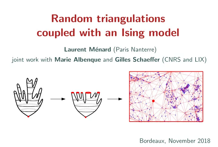
Laurent M´ enard (Paris Nanterre) joint work with Marie Albenque and Gilles Schaeffer (CNRS and LIX) Bordeaux, November 2018

Outline

• 1. Introduction: 2DQG and planar maps
• 2. Local weak topology
• 3. Adding matter: Ising model
• 4. Combinatorics of triangulations with spins
• 5. Local limit of triangulations with spins

2D Quantum Gravity?

[Polyakov 81] ”We have to develop an art of handling sums over random surfaces. These sums replace the old fashioned (and extremely useful) sums over random paths.”

2D Quantum Gravity?

[Polyakov 81] ”We have to develop an art of handling sums over random surfaces. These sums replace the old fashioned (and extremely useful) sums over random paths.” Sums over random paths: Feynman path integrals. Well understood question: Pick a, b ∈ R2, what does a random path γ : [0, 1] → R2 chosen ”uniformly at random” between all paths from a to b look like?

2D Quantum Gravity?

[Polyakov 81] ”We have to develop an art of handling sums over random surfaces. These sums replace the old fashioned (and extremely useful) sums over random paths.” Sums over random paths: Feynman path integrals. Well understood question: Pick a, b ∈ R2, what does a random path γ : [0, 1] → R2 chosen ”uniformly at random” between all paths from a to b look like? Brownian motion!

2D Quantum Gravity?

[Polyakov 81] ”We have to develop an art of handling sums over random surfaces. These sums replace the old fashioned (and extremely useful) sums over random paths.” Sums over random paths: Feynman path integrals. Well understood question: Pick a, b ∈ R2, what does a random path γ : [0, 1] → R2 chosen ”uniformly at random” between all paths from a to b look like? Brownian motion! Not so well understood question: What does a random metric on S2 distributed ”uniformly” look like? Brownian surface?

2D Quantum Gravity?

[Polyakov 81] ”We have to develop an art of handling sums over random surfaces. These sums replace the old fashioned (and extremely useful) sums over random paths.” Sums over random paths: Feynman path integrals. Well understood question: Pick a, b ∈ R2, what does a random path γ : [0, 1] → R2 chosen ”uniformly at random” between all paths from a to b look like? Brownian motion! Not so well understood question: What does a random metric on S2 distributed ”uniformly” look like? Brownian surface? First idea: try discrete metric spaces (Donsker)

Planar Maps as discrete planar metric spaces

Definition: A planar map is a proper embedding of a finite connected graph into the two-dimensional sphere (considered up to orientation-preserving homeomorphisms of the sphere).

Planar Maps as discrete planar metric spaces

Definition: A planar map is a proper embedding of a finite connected graph into the two-dimensional sphere (considered up to orientation-preserving homeomorphisms of the sphere). = = =

Planar Maps as discrete planar metric spaces

Definition: A planar map is a proper embedding of a finite connected graph into the two-dimensional sphere (considered up to orientation-preserving homeomorphisms of the sphere). faces: connected components of the complement of edges p-angulation: each face is bounded by p edges = = =

Planar Maps as discrete planar metric spaces

Definition: A planar map is a proper embedding of a finite connected graph into the two-dimensional sphere (considered up to orientation-preserving homeomorphisms of the sphere). faces: connected components of the complement of edges p-angulation: each face is bounded by p edges

Planar Maps as discrete planar metric spaces

Definition: A planar map is a proper embedding of a finite connected graph into the two-dimensional sphere (considered up to orientation-preserving homeomorphisms of the sphere). faces: connected components of the complement of edges p-angulation: each face is bounded by p edges

Planar Maps as discrete planar metric spaces

Definition: A planar map is a proper embedding of a finite connected graph into the two-dimensional sphere (considered up to orientation-preserving homeomorphisms of the sphere). faces: connected components of the complement of edges p-angulation: each face is bounded by p edges This is a triangulation

Planar Maps as discrete planar metric spaces

Definition: A planar map is a proper embedding of a finite connected graph into the two-dimensional sphere (considered up to orientation-preserving homeomorphisms of the sphere). M Planar Map:

• V (M) := set of vertices of M
• dgr := graph distance on V (M)
• (V (M), dgr) is a (finite) metric space

In blue, distances from 1 1 1 1 1 1 1 2

Planar Maps as discrete planar metric spaces

Definition: A planar map is a proper embedding of a finite connected graph into the two-dimensional sphere (considered up to orientation-preserving homeomorphisms of the sphere). M Planar Map:

• V (M) := set of vertices of M
• dgr := graph distance on V (M)
• (V (M), dgr) is a (finite) metric space

In blue, distances from 1 1 1 1 1 1 1 2 Rooted map: mark an oriented edge of the map

”Classical” large random triangulations

Take a triangulation of size n uniformly at random. What does it look like if n is large ? Two points of view: global/local, continuous/discrete Euler relation in a triangulation: number of edges / vertices / faces linked

”Classical” large random triangulations

Take a triangulation of size n uniformly at random. What does it look like if n is large ? Two points of view: global/local, continuous/discrete Global : Rescale distances to keep diameter bounded [Le Gall 13, Miermont 13]: converges to the Brownian map.

• Gromov-Hausdorff topology
• Continuous metric space
• Homeomorphic to the sphere
• Hausdorff dimension 4
• Universality

Euler relation in a triangulation: number of edges / vertices / faces linked

”Classical” large random triangulations

Take a triangulation of size n uniformly at random. What does it look like if n is large ? Two points of view: global/local, continuous/discrete Local : Don’t rescale distances and look at neighborhoods of the root Euler relation in a triangulation: number of edges / vertices / faces linked

”Classical” large random triangulations

Take a triangulation of size n uniformly at random. What does it look like if n is large ? Two points of view: global/local, continuous/discrete Local : Don’t rescale distances and look at neighborhoods of the root [Angel – Schramm 03, Krikun 05]: Converges to the Uniform Infinite Planar Triangulation

• Local topology
• Metric balls of radius R grow like R4
• ”Universality” of the exponent 4.

Euler relation in a triangulation: number of edges / vertices / faces linked

Local Topology for planar maps

Mf := {finite rooted planar maps}. Definition: The local topology on Mf is induced by the distance: dloc(m, m′) := (1 + max{r ≥ 0 : Br(m) = Br(m′)})−1 where Br(m) is the graph made of all the vertices and edges of m which are within distance r from the root.

Local Topology for planar maps

Mf := {finite rooted planar maps}. Definition: The local topology on Mf is induced by the distance: dloc(m, m′) := (1 + max{r ≥ 0 : Br(m) = Br(m′)})−1 where Br(m) is the graph made of all the vertices and edges of m which are within distance r from the root.

• (M, dloc): closure of (Mf, dloc). It is a Polish space

(complete and separable).

• M∞ := M \ Mf set of infinite planar maps.

Local convergence: simple examples

1 2 n Root = 0

Local convergence: simple examples

1 2 n − → (Z+, 0) Root = 0

Local convergence: simple examples

1 2 n − → (Z+, 0) Root = 0 1 2 n Uniformly chosen root

Local convergence: simple examples

1 2 n − → (Z+, 0) Root = 0 1 2 n Uniformly chosen root

Local convergence: simple examples

1 2 n − → (Z+, 0) Root = 0 1 2 n − → (Z, 0) Uniformly chosen root

Local convergence: simple examples

1 2 n − → (Z+, 0) 1 2 n − → (Z, 0) Root = 0 1 2 n − → (Z, 0) Uniformly chosen root Root does not matter

Local convergence: simple examples

1 2 n − → (Z+, 0) 1 2 n − → (Z, 0) n n − →

• Z2

+, 0

• Root = 0

1 2 n − → (Z, 0) Uniformly chosen root Root does not matter

Local convergence: simple examples

1 2 n − → (Z+, 0) 1 2 n − → (Z, 0) n n − →

• Z2

+, 0

• Root = 0

1 2 n − → (Z, 0) Uniformly chosen root Root does not matter n n − →

• Z2, 0
• Uniformly chosen root

Local convergence: more complicated examples

Uniform plane rooted trees with n vertices:

n = 1 n = 2 n = 4 n = 3 1/2 1/2 1/5 1/5 1/5 1/5 1/5

Local convergence: more complicated examples

Uniform plane rooted trees with n vertices:

n = 1 n = 2 n = 4 n = 3 1/2 1/2 1/5 1/5 1/5 1/5 1/5 n = 1000 n = 500

Local convergence: more complicated examples

Uniform plane rooted trees with n vertices:

n = 1 n = 2 n = 4 n = 3 1/2 1/2 1/5 1/5 1/5 1/5 1/5 n = 1000 n = 500

The limit is a probability distribution on infinite trees with one infinite branch.

Local convergence of uniform triangulations

Theorem [Angel – Schramm, ’03] As n → ∞, the uniform distribution on triangulations of size n converges weakly to a probability measure called the Uniform Infinite Planar Triangulation (or UIPT) for the local topology.

Courtesy of Timothy Budd Courtesy of Igor Kortchemski

Local convergence of uniform triangulations

Theorem [Angel – Schramm, ’03] As n → ∞, the uniform distribution on triangulations of size n converges weakly to a probability measure called the Uniform Infinite Planar Triangulation (or UIPT) for the local topology. Some properties of the UIPT:

• Volume (nb. of vertices) and perimeters of balls known to some extent.

For example E [|Br(T∞)|] ∼ 2 7r4 [Angel ’04, Curien – Le Gall ’12]

• Simple random Walk is recurrent [Gurel-Gurevich and Nachmias ’13]
• The UIPT has almost surely one end [Angel – Schramm, ’03]
• Volume of hulls explicit [M. 16]
• ”Uniqueness” of geodesic rays and horofunctions [Curien – M. 18]
• Bond and site percolation well understood [Angel, Angel–Curien, M.–Nolin]

Local convergence of uniform triangulations

Theorem [Angel – Schramm, ’03] As n → ∞, the uniform distribution on triangulations of size n converges weakly to a probability measure called the Uniform Infinite Planar Triangulation (or UIPT) for the local topology. Some properties of the UIPT:

• Volume (nb. of vertices) and perimeters of balls known to some extent.

For example E [|Br(T∞)|] ∼ 2 7r4 [Angel ’04, Curien – Le Gall ’12]

• Simple random Walk is recurrent [Gurel-Gurevich and Nachmias ’13]

Universality: we expect the same behavior for slightly different models (e.g. quadrangulations, triangulations without loops, ...)

• The UIPT has almost surely one end [Angel – Schramm, ’03]
• Volume of hulls explicit [M. 16]
• ”Uniqueness” of geodesic rays and horofunctions [Curien – M. 18]
• Bond and site percolation well understood [Angel, Angel–Curien, M.–Nolin]

Adding matter: Ising model on triangulations

How does Ising model influence the underlying map?

Adding matter: Ising model on triangulations

How does Ising model influence the underlying map? First, Ising model on a finite deterministic graph: G = (V, E) finite graph Spin configuration on G: σ : V → {−1, +1}.

− + + − − −

Adding matter: Ising model on triangulations

How does Ising model influence the underlying map? First, Ising model on a finite deterministic graph: G = (V, E) finite graph Spin configuration on G: σ : V → {−1, +1}.

− + + − − −

Ising model on G: take a random spin configuration with probability P(σ) ∝ e− β

2

• v∼v′ 1{σ(v)=σ(v′)}

β > 0: inverse temperature.

Adding matter: Ising model on triangulations

How does Ising model influence the underlying map? First, Ising model on a finite deterministic graph: G = (V, E) finite graph Spin configuration on G: σ : V → {−1, +1}.

− + + − − −

Ising model on G: take a random spin configuration with probability P(σ) ∝ e− β

2

• v∼v′ 1{σ(v)=σ(v′)}

β > 0: inverse temperature. Combinatorial formulation: P(σ) ∝ νm(σ) with m(σ) = number of monochromatic edges and ν = eβ. m(σ) = 4 m(σ) = 4

Adding matter: Ising model on triangulations

Tn = {rooted planar triangulations with 3n edges}. Random triangulation in Tn with probability ∝ νm(T,σ) ?

Adding matter: Ising model on triangulations

Tn = {rooted planar triangulations with 3n edges}. Generating series of Ising-weighted triangulations: Q(ν, t) =

• T ∈Tf
• σ:V (T )→{−1,+1}

νm(T,σ)te(T ). Random triangulation in Tn with probability ∝ νm(T,σ) ?

Adding matter: Ising model on triangulations

Tn = {rooted planar triangulations with 3n edges}. Generating series of Ising-weighted triangulations: Q(ν, t) =

• T ∈Tf
• σ:V (T )→{−1,+1}

νm(T,σ)te(T ). Theorem [Bernardi – Bousquet-M´ elou 11] For every ν the series Q(ν, t) is algebraic, has ρν > 0 as unique dominant singularity and satisfies [t3n]Q(ν, t) ∼

n→∞

• κ ρ−n

νc n−7/3

if ν = νc := 1 +

1 √ 7,

κ ρ−n

ν

n−5/2 if ν = νc. This suggests an unusual behavior of the underlying maps for ν = νc. Random triangulation in Tn with probability ∝ νm(T,σ) ? See also [Boulatov – Kazakov 1987], [Bousquet-M´ elou – Schaeffer 03] and [Bouttier – Di Francesco – Guitter 04].

Adding matter: the model and Watabiki’s predictions

Pν

n

• {(T, σ)}
• =

νm(T,σ) [t3n]Q(ν, t). Probability measure on triangulations of Tn with a spin configuration:

Adding matter: the model and Watabiki’s predictions

Counting exponent: coeff [tn] of generating series of (decorated) maps ∼ κρ−nn−α Central charge c: α = 25 − c +

• (1 − c)(25 − c)

12 Hausdorff dimension: [Watabiki 93] DH = 2 √25 − c + √49 − c √25 − c + √1 − c Pν

n

• {(T, σ)}
• =

νm(T,σ) [t3n]Q(ν, t). Probability measure on triangulations of Tn with a spin configuration:

Adding matter: the model and Watabiki’s predictions

Counting exponent: coeff [tn] of generating series of (decorated) maps ∼ κρ−nn−α Central charge c: α = 25 − c +

• (1 − c)(25 − c)

12 Hausdorff dimension: [Watabiki 93]

• α = 5/2 gives DH = 4
• α = 7/3 gives DH = 7+

√ 97 4

≈ 4.21 DH = 2 √25 − c + √49 − c √25 − c + √1 − c Pν

n

• {(T, σ)}
• =

νm(T,σ) [t3n]Q(ν, t). Probability measure on triangulations of Tn with a spin configuration:

Local Topology for planar maps : balls

Definition: The local topology on Tf is induced by the distance: dloc(T, T ′) := (1 + max{r ≥ 0 : Br(T) = Br(T ′)})−1 where Br(T) is the submap (with spins) of T composed by the faces

• f T with a vertex at distance < r from the root.

Local Topology for planar maps : balls

Definition: The local topology on Tf is induced by the distance:

1 1 1 1 1 2 2 2 2 2 2 3 3 2 4 4 4 4 4 4 4 5 5 2 2 2 2 2 3 3 3 3 1 3 3 4 4 4 4 4 4 4 4 4

dloc(T, T ′) := (1 + max{r ≥ 0 : Br(T) = Br(T ′)})−1 where Br(T) is the submap (with spins) of T composed by the faces

• f T with a vertex at distance < r from the root.

Local Topology for planar maps : balls

Definition: The local topology on Tf is induced by the distance:

1 1 1 1 1 2 2 2 2 2 2 3 3 2 4 4 4 4 4 4 4 5 5 2 2 2 2 2 3 3 3 3 1 3 3 4 4 4 4 4 4 4 4 4

dloc(T, T ′) := (1 + max{r ≥ 0 : Br(T) = Br(T ′)})−1 where Br(T) is the submap (with spins) of T composed by the faces

• f T with a vertex at distance < r from the root.

Local Topology for planar maps : balls

Definition: The local topology on Tf is induced by the distance:

1 1 1 1 1 2 2 2 2 2 2 3 3 2 4 4 4 4 4 4 4 5 5 2 2 2 2 2 3 3 3 3 1 3 3 4 4 4 4 4 4 4 4 4

dloc(T, T ′) := (1 + max{r ≥ 0 : Br(T) = Br(T ′)})−1 where Br(T) is the submap (with spins) of T composed by the faces

• f T with a vertex at distance < r from the root.

Local Topology for planar maps : balls

Definition: The local topology on Tf is induced by the distance:

1 1 1 1 1 2 2 2 2 2 2 3 3 2 4 4 4 4 4 4 4 5 5 2 2 2 2 2 3 3 3 3 1 3 3 4 4 4 4 4 4 4 4 4

dloc(T, T ′) := (1 + max{r ≥ 0 : Br(T) = Br(T ′)})−1 where Br(T) is the submap (with spins) of T composed by the faces

• f T with a vertex at distance < r from the root.

Local Topology for planar maps : balls

Definition: The local topology on Tf is induced by the distance:

1 1 1 1 1 2 2 2 2 2 2 3 3 2 4 4 4 4 4 4 4 5 5 2 2 2 2 2 3 3 3 3 1 3 3 4 4 4 4 4 4 4 4 4

dloc(T, T ′) := (1 + max{r ≥ 0 : Br(T) = Br(T ′)})−1 where Br(T) is the submap (with spins) of T composed by the faces

• f T with a vertex at distance < r from the root.

Local Topology for planar maps : balls

Definition: The local topology on Tf is induced by the distance: dloc(T, T ′) := (1 + max{r ≥ 0 : Br(T) = Br(T ′)})−1 where Br(T) is the submap (with spins) of T composed by the faces

• f T with a vertex at distance < r from the root.

r T Br(T) simple cycles

• (T , dloc): closure of (Tf, dloc).

It is a Polish space.

• T∞ := T \ Tf set of infinite planar

triangulations.

Weak convergence for the local topology

Portemanteau theorem + Levy – Prokhorov metric: A sequence of measures measures (Pn) on Tf converge weakly to a measure P on T∞ if: Pn

• {(T, v) ∈ Tf : Br(T, v) = ∆}
• −

→

n→∞ P

• {T ∈ T∞ : Br(T) = ∆}
• .
• 1. For every r > 0 and every possible r-ball ∆

Weak convergence for the local topology

Portemanteau theorem + Levy – Prokhorov metric: A sequence of measures measures (Pn) on Tf converge weakly to a measure P on T∞ if: Pn

• {(T, v) ∈ Tf : Br(T, v) = ∆}
• −

→

n→∞ P

• {T ∈ T∞ : Br(T) = ∆}
• .

degree n

• 1. For every r > 0 and every possible r-ball ∆

Problem: not sufficient since the space (T , dloc) is not compact! Ex:

Weak convergence for the local topology

Portemanteau theorem + Levy – Prokhorov metric: A sequence of measures measures (Pn) on Tf converge weakly to a measure P on T∞ if: Pn

• {(T, v) ∈ Tf : Br(T, v) = ∆}
• −

→

n→∞ P

• {T ∈ T∞ : Br(T) = ∆}
• .
• 2. No loss of mass at the limit: Tightness of (Pn), or

the measure P defined by the limits in 1. is a probability measure.

• 1. For every r > 0 and every possible r-ball ∆

∀r > 0,

• r−balls ∆

P

• {T ∈ T∞ : Br(T) = ∆}
• = 1.
• Vertex degrees are tight (at finite distance from the root)

Local convergence and generating series

Need to evaluate, for every possible ball ∆ (here, one boundary to keep it simple) Pn ∆ ???

Local convergence and generating series

Need to evaluate, for every possible ball ∆ (here, one boundary to keep it simple) Pn ∆ ???

• Simple (rooted) cycle,

spins given by a word ω

Local convergence and generating series

Need to evaluate, for every possible ball ∆ (here, one boundary to keep it simple) Pn ∆ ???

• Simple (rooted) cycle,

spins given by a word ω = νm(∆)−m(ω) [t3n−e(∆)+|ω|]Zω(ν, t) [t3n]Q(ν, t) Zω(ν, t) := generating series of triangulations with simple boundary ω

Local convergence and generating series

Theorem [Albenque – M. – Schaeffer 18+] For every ω and ν, the series t|ω|Zω(ν, t) is algebraic, has ρν = t3

ν as

unique dominant singularity and satisfies Need to evaluate, for every possible ball ∆ (here, one boundary to keep it simple) Pn ∆ ???

• Simple (rooted) cycle,

spins given by a word ω = νm(∆)−m(ω) [t3n−e(∆)+|ω|]Zω(ν, t) [t3n]Q(ν, t) Zω(ν, t) := generating series of triangulations with simple boundary ω [t3n]t|ω|Zω(ν, t) ∼

n→∞

• κω(νc) ρ−n

νc n−7/3

if ν = νc := 1 +

1 √ 7,

κω(ν) ρ−n

ν

n−5/2 if ν = νc.

Triangulations with simple boundary

To get exact asymptotics we need, as series in t3,

• 1. algebraicity,
• 2. no other dominant singularity than ρν.

Fix a word ω, with injections from and into triangulations of the sphere: [t3n]t|ω|Zω = Θ

• ρ−n

ν n−α

, with α = 5/2 of 7/3 depending on ν.

Triangulations with simple boundary

= +

• a

a Zω

• Z⊕ω

+ Z⊖ω +

• ω=ω1aω2

Zaω1 ·Zaω2

• =

× ν1←

− ω =− → ω t

Tutte’s equation (or peeling equation, or loop equation... ): To get exact asymptotics we need, as series in t3,

• 1. algebraicity,
• 2. no other dominant singularity than ρν.

Fix a word ω, with injections from and into triangulations of the sphere: [t3n]t|ω|Zω = Θ

• ρ−n

ν n−α

, with α = 5/2 of 7/3 depending on ν.

Triangulations with simple boundary

= +

• a

a Zω

• Z⊕ω

+ Z⊖ω +

• ω=ω1aω2

Zaω1 ·Zaω2

• =

× ν1←

− ω =− → ω t

Tutte’s equation (or peeling equation, or loop equation... ): Double induction on |ω| and number of ⊖’s: enough to prove 1. and 2. for the tpZ⊕p’s To get exact asymptotics we need, as series in t3,

• 1. algebraicity,
• 2. no other dominant singularity than ρν.

Fix a word ω, with injections from and into triangulations of the sphere: [t3n]t|ω|Zω = Θ

• ρ−n

ν n−α

, with α = 5/2 of 7/3 depending on ν.

Positive boundary conditions: two catalytic variables

= +

• A(x) :=
• p≥1

Z⊕pxp = + νtx2+ +νt x (A(x))2

Positive boundary conditions: two catalytic variables

= +

• Peeling equation at interface ⊖–⊕:

= +

• A(x) :=
• p≥1

Z⊕pxp = + νtx2+ +νt x (A(x))2 S(x, y) :=

• p,q≥1

Z⊕p⊖qxpyq +

Positive boundary conditions: two catalytic variables

= +

• Peeling equation at interface ⊖–⊕:

= +

• A(x) :=
• p≥1

Z⊕pxp = + νtx2+ +νt x (A(x))2 S(x, y) :=

• p,q≥1

Z⊕p⊖qxpyq + νt x

• A(x)−xZ⊕
• +νt [y]S(x, y)

Positive boundary conditions: two catalytic variables

= +

• Peeling equation at interface ⊖–⊕:

= +

• A(x) :=
• p≥1

Z⊕pxp = + νtx2+ +νt x (A(x))2 S(x, y) :=

• p,q≥1

Z⊕p⊖qxpyq + νt x

• A(x)−xZ⊕
• +νt [y]S(x, y)

= txy+ t x

• S(x, y)−x[x]S(x, y)
• + t

y

• S(x, y)−y[y]S(x, y)
• + t

xS(x, y)A(x) + t y S(x, y)A(y)

From two catalytic variables to one: Tutte’s invariants

Kernel method: equation for S reads K(x, y) · S(x, y) = R(x, y) K(x, y) = 1 − t x − t y − t xA(x) − t y A(y). where

From two catalytic variables to one: Tutte’s invariants

Kernel method: equation for S reads K(x, y) · S(x, y) = R(x, y) K(x, y) = 1 − t x − t y − t xA(x) − t y A(y). where

• 1. Find two series Y1 and Y2 in Q(x)[[t]] such that K(x, Yi/t) = 0.

From two catalytic variables to one: Tutte’s invariants

Kernel method: equation for S reads K(x, y) · S(x, y) = R(x, y) K(x, y) = 1 − t x − t y − t xA(x) − t y A(y). where

• 1. Find two series Y1 and Y2 in Q(x)[[t]] such that K(x, Yi/t) = 0.

It gives

1 Y1 (A(Y1/t) + 1) = 1 Y2 (A(Y2/t) + 1).

From two catalytic variables to one: Tutte’s invariants

Kernel method: equation for S reads K(x, y) · S(x, y) = R(x, y) K(x, y) = 1 − t x − t y − t xA(x) − t y A(y). where

• 1. Find two series Y1 and Y2 in Q(x)[[t]] such that K(x, Yi/t) = 0.

It gives

1 Y1 (A(Y1/t) + 1) = 1 Y2 (A(Y2/t) + 1).

I(y) := 1

y (A(y/t) + 1) is called an invariant.

From two catalytic variables to one: Tutte’s invariants

Kernel method: equation for S reads K(x, y) · S(x, y) = R(x, y) K(x, y) = 1 − t x − t y − t xA(x) − t y A(y). where

• 1. Find two series Y1 and Y2 in Q(x)[[t]] such that K(x, Yi/t) = 0.

It gives

1 Y1 (A(Y1/t) + 1) = 1 Y2 (A(Y2/t) + 1).

I(y) := 1

y (A(y/t) + 1) is called an invariant.

• 2. Work a bit with the help of R(x, Yi/t) = 0 to get a second invariant

J(y) depending only on t, Z⊕(t), y and A(y/t).

From two catalytic variables to one: Tutte’s invariants

Kernel method: equation for S reads K(x, y) · S(x, y) = R(x, y) K(x, y) = 1 − t x − t y − t xA(x) − t y A(y). where

• 1. Find two series Y1 and Y2 in Q(x)[[t]] such that K(x, Yi/t) = 0.

It gives

1 Y1 (A(Y1/t) + 1) = 1 Y2 (A(Y2/t) + 1).

I(y) := 1

y (A(y/t) + 1) is called an invariant.

• 2. Work a bit with the help of R(x, Yi/t) = 0 to get a second invariant

J(y) depending only on t, Z⊕(t), y and A(y/t).

• 3. Prove that J(y) = C0(t) + C1(t)I(y) + C2(t)I2(y) with Ci’s explicit

polynomials in t, Z⊕(t) and Z⊕2(t). Equation with one catalytic variable for A(y) with Z⊕ and Z⊕2 !

Explicit solution for positive boundary conditions

2t2ν(1 − ν) A(y) y − Z⊕

• = y · Pol
• ν, A(y)

y , Z⊕, Z⊕2, t, y

• Equation with one catalytic variable reads:

[Bousquet-M´ elou – Jehanne 06] gives algebraicity and strategy to solve this kind of equation.

Explicit solution for positive boundary conditions

2t2ν(1 − ν) A(y) y − Z⊕

• = y · Pol
• ν, A(y)

y , Z⊕, Z⊕2, t, y

• Equation with one catalytic variable reads:

[Bousquet-M´ elou – Jehanne 06] gives algebraicity and strategy to solve this kind of equation. Much easier: [Bernardi – Bousquet M´ elou 11] gives us Z⊕ and Z⊕2!

Explicit solution for positive boundary conditions

2t2ν(1 − ν) A(y) y − Z⊕

• = y · Pol
• ν, A(y)

y , Z⊕, Z⊕2, t, y

• Equation with one catalytic variable reads:

[Bousquet-M´ elou – Jehanne 06] gives algebraicity and strategy to solve this kind of equation. Much easier: [Bernardi – Bousquet M´ elou 11] gives us Z⊕ and Z⊕2!

t3 = U P1(µ, U) 4(1 − 2U)2(1 + µ)3 y = V P2(µ, U, V ) (1 − 2U)(1 + µ)2(1 − V )2 t3A(t, ty) = V P3(µ, U, V ) 4(1 − 2U)2(1 + µ)3(1 − V )3

Maple: rational (and Lagrangian) parametrization ! with ν = 1+µ

1−µ and

Pi’s explicit polynomials.

Going back to local convergence

Pn (Br(T, v) = ∆) = νm(∆)−m(∂∆) [t3n−e(∆)+|∂∆|] k

i=1 Zωi(ν, t)

• [t3n]Q(ν, t)

→

n→∞

k

• i=1

Zωi(ν, tν)

• ·

k

• j=1

νm(∆)−m(∂∆) t|∆|−|ω|

ν

κωj κ t|ωj|

ν

Zωj(ν, tν) .

• 1. Fix r ≥ 0 and take ∆ a r-ball with boundary spins ∂∆ = (ω1, . . . , ωk):

Going back to local convergence

Pn (Br(T, v) = ∆) = νm(∆)−m(∂∆) [t3n−e(∆)+|∂∆|] k

i=1 Zωi(ν, t)

• [t3n]Q(ν, t)

→

n→∞

k

• i=1

Zωi(ν, tν)

• ·

k

• j=1

νm(∆)−m(∂∆) t|∆|−|ω|

ν

κωj κ t|ωj|

ν

Zωj(ν, tν) .

• 2. Remains to prove tightness.
• 1. Fix r ≥ 0 and take ∆ a r-ball with boundary spins ∂∆ = (ω1, . . . , ωk):

Going back to local convergence

Pn (Br(T, v) = ∆) = νm(∆)−m(∂∆) [t3n−e(∆)+|∂∆|] k

i=1 Zωi(ν, t)

• [t3n]Q(ν, t)

→

n→∞

k

• i=1

Zωi(ν, tν)

• ·

k

• j=1

νm(∆)−m(∂∆) t|∆|−|ω|

ν

κωj κ t|ωj|

ν

Zωj(ν, tν) .

• 2. Remains to prove tightness.
• 1. Fix r ≥ 0 and take ∆ a r-ball with boundary spins ∂∆ = (ω1, . . . , ωk):
• Maps are uniformly rooted:

tightness of root degree is enough

Going back to local convergence

Pn (Br(T, v) = ∆) = νm(∆)−m(∂∆) [t3n−e(∆)+|∂∆|] k

i=1 Zωi(ν, t)

• [t3n]Q(ν, t)

→

n→∞

k

• i=1

Zωi(ν, tν)

• ·

k

• j=1

νm(∆)−m(∂∆) t|∆|−|ω|

ν

κωj κ t|ωj|

ν

Zωj(ν, tν) .

• 2. Remains to prove tightness.
• 1. Fix r ≥ 0 and take ∆ a r-ball with boundary spins ∂∆ = (ω1, . . . , ωk):
• Maps are uniformly rooted:

tightness of root degree is enough

• We show that expected degree at the root

under Pn is bounded with n

A simple tightness argument

Pn (δ ∈ e) =

3n

• k=1

P (δ ∈ e|deg(δ) = k) · Pn (deg(δ) = k) ≥

3n

• k=1

k 2 · 3nPn (deg(δ) = k) = 1 6nEn [deg(δ)] Mark a uniform edge conditionally on the triangulation We want to study the degree of the root vertex δ:

A simple tightness argument

Pn (δ ∈ e) =

3n

• k=1

P (δ ∈ e|deg(δ) = k) · Pn (deg(δ) = k) ≥

3n

• k=1

k 2 · 3nPn (deg(δ) = k) = 1 6nEn [deg(δ)] Pn (δ ∈ e) ≤ max 1 ν , 1 2 [t3n+2](Z4 + Z2

2 + Z2 1 + Z2 1Z2 + Z1Z3)

3n [t3n]Z = O(1/n) Mark a uniform edge conditionally on the triangulation We want to study the degree of the root vertex δ: Cut open the marked edge and the root:

A simple tightness argument

Pn (δ ∈ e) =

3n

• k=1

P (δ ∈ e|deg(δ) = k) · Pn (deg(δ) = k) ≥

3n

• k=1

k 2 · 3nPn (deg(δ) = k) = 1 6nEn [deg(δ)] Pn (δ ∈ e) ≤ max 1 ν , 1 2 [t3n+2](Z4 + Z2

2 + Z2 1 + Z2 1Z2 + Z1Z3)

3n [t3n]Z = O(1/n) Mark a uniform edge conditionally on the triangulation We want to study the degree of the root vertex δ: Cut open the marked edge and the root: En [deg(δ)] = O(1).

The story so far

What we know:

• Convergence in law for the local toplogy.
• The limiting random triangulation has one end a.s.

The story so far

What we know:

• Convergence in law for the local toplogy.
• The limiting random triangulation has one end a.s.
• A spatial Markov property.
• Some links with Boltzmann triangulations.

The story so far

What we know:

• Convergence in law for the local toplogy.
• The limiting random triangulation has one end a.s.
• A spatial Markov property.
• Some links with Boltzmann triangulations.
• Recurrence of SRW (vertex degrees have exponential tails)
• Cluster properties.

In progress:

The story so far

What we know:

• Convergence in law for the local toplogy.
• The limiting random triangulation has one end a.s.

What we would like to know:

• Singularity with respect to the UIPT?
• Volume growth?
• A spatial Markov property.
• Some links with Boltzmann triangulations.
• Recurrence of SRW (vertex degrees have exponential tails)
• Cluster properties.

In progress:

The story so far

What we know:

• Convergence in law for the local toplogy.
• The limiting random triangulation has one end a.s.

What we would like to know:

• Singularity with respect to the UIPT?
• Volume growth?
• At least volume growth = 4 at νc?
• A spatial Markov property.
• Some links with Boltzmann triangulations.
• Recurrence of SRW (vertex degrees have exponential tails)
• Cluster properties.

In progress:

Summer school Random trees and graphs July 1 to 5, 2019 in Marseille France

• Org. M. Albenque, J. Bettinelli, J. Ru´

e and L.Menard

Thank you for your attention!

Summer school Random walks and models of complex networks July 8 to 19, 2019 in Nice

• Org. B. Reed and D. Mitsche