Review: Case where index is useful Query Optimization in Relational - - PDF document

review case where index is useful
SMART_READER_LITE
LIVE PREVIEW

Review: Case where index is useful Query Optimization in Relational - - PDF document

Review: Case where index is useful Query Optimization in Relational Database Systems It is safer to accept any chance It is safer to accept any chance that offers itself, and extemporize a procedure to fit it, than to get a good plan matured,


slide-1
SLIDE 1

1 Query Optimization in Relational Database Systems

It is safer to accept any chance

CS5208: Query Optimization 1

It is safer to accept any chance that offers itself, and extemporize a procedure to fit it, than to get a good plan matured, and wait for a chance of using it. Thomas Hardy (1874) in Far from the Madding Crowd

Review: Case where index is useful

CS5208: Query Optimization 2

Query Optimization

  • Since each relational op returns a relation, ops can be

composed!

  • Queries that require multiple ops to be composed may

be composed in different ways - thus optimization is necessary for good performance e g A B C D can

CS5208: Query Optimization 3

necessary for good performance, e.g. A B C D can be evaluated as follows:

  • (((A B) C) D)
  • ((A B) (C D))
  • ((B A) (D C))

Query Optimization

  • Each strategy can be represented as a query

evaluation plan (QEP) - Tree of R.A. ops, with choice

  • f algo for each op.

D NL SM HJ

CS5208: Query Optimization 4

  • Goal of optimization: To find the “best” plan that

compute the same answer (to avoid “bad” plans)

A B C D A B C D NL NL HJ INL

More on Motivating Examples

Sailors (sid: integer, sname: string, rating: integer, age: real) Reserves (sid: integer, bid: integer, day: dates, rname: string)

CS5208: Query Optimization 5

  • Reserves:
  • Each tuple is 40 bytes long, 100 tuples per page, 1000 pages.
  • Sailors:
  • Each tuple is 50 bytes long, 80 tuples per page, 500 pages.
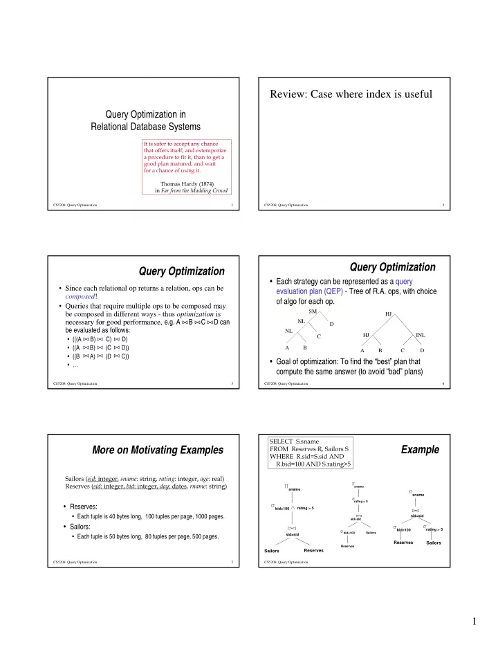
Example

SELECT S.sname FROM Reserves R, Sailors S WHERE R.sid=S.sid AND R.bid=100 AND S.rating>5

sname sname

sname ti > 5

CS5208: Query Optimization

Sailors Reserves

sid=sid bid=100 rating > 5

Reserves Sailors

sid=sid bid=100 rating > 5

Reserves Sailors sid=sid bid=100 rating > 5

slide-2
SLIDE 2

2

Example

SELECT S.sname FROM Reserves R, Sailors S WHERE R.sid=S.sid AND R.bid=100 AND S.rating>5

sname sid sname rating age bid day rname sname lubber CS5208: Query Optimization

Sailors Reserves

sid=sid bid=100 rating > 5 sid sname rating age 22 dustin 7 45.0 28 yuppy 9 35.0 31 lubber 8 55.5 44 guppy 5 35.0 58 rusty 10 35.0 sid bid day rname 31 100 10/11/96 lubber 58 103 11/12/96 dustin sid sname rating age bid day rname 31 lubber 8 55.5 100 10/11/96 lubber 58 rusty 10 35.0 103 11/12/96 dustin 31 lubber 8 55.5 100 10/11/96 lubber

Example

SELECT S.sname FROM Reserves R, Sailors S WHERE R.sid=S.sid AND R.bid=100 AND S.rating>5

sname rating > 5 sname lubber sid sname rating age bid day rname 31 lubber 8 55.5 100 10/11/96 lubber

CS5208: Query Optimization

Reserves Sailors sid=sid bid=100 rating 5

sid sname rating age 22 dustin 7 45.0 28 yuppy 9 35.0 31 lubber 8 55.5 44 guppy 5 35.0 58 rusty 10 35.0 sid bid day rname 31 100 10/11/96 lubber 58 103 11/12/96 dustin sid sname rating age bid day rname 31 lubber 8 55.5 100 10/11/96 lubber sid bid day rname 31 100 10/11/96 lubber 31 lubber 8 55.5 100 10/11/96 lubber

Example

SELECT S.sname FROM Reserves R, Sailors S WHERE R.sid=S.sid AND R.bid=100 AND S.rating>5

sname sid sname rating age bid day rname 31 lubber 8 55.5 100 10/11/96 lubber sname lubber CS5208: Query Optimization

Reserves Sailors

sid=sid bid=100 rating > 5 sid sname rating age 22 dustin 7 45.0 28 yuppy 9 35.0 31 lubber 8 55.5 44 guppy 5 35.0 58 rusty 10 35.0 sid bid day rname 31 100 10/11/96 lubber 58 103 11/12/96 dustin 31 lubber 8 55.5 100 10/11/96 lubber sid bid day rname 31 100 10/11/96 lubber sid sname rating age 22 dustin 7 45.0 28 yuppy 9 35.0 31 lubber 8 55.5 58 rusty 10 35.0

Example (Cont)

SELECT S.sname FROM Reserves R, Sailors S WHERE R.sid=S.sid AND R.bid=100 AND S.rating>5

sname

(On-the-fly)

Query Evaluation Plan:

  • Cost?

CS5208: Query Optimization 10

Sailors Reserves

sid=sid bid=100 rating > 5

(Page Nested Loops) (On-the-fly)

Example (Cont)

SELECT S.sname FROM Reserves R, Sailors S WHERE R.sid=S.sid AND R.bid=100 AND S.rating>5

sname

(On-the-fly)

Query Evaluation Plan:

  • Cost: 500+500*1000 I/Os

CS5208: Query Optimization 11

Sailors Reserves

sid=sid bid=100 rating > 5

(Page Nested Loops) (On-the-fly)

Example (Cont)

SELECT S.sname FROM Reserves R, Sailors S WHERE R.sid=S.sid AND R.bid=100 AND S.rating>5

sname

(On-the-fly)

Query Evaluation Plan:

  • Cost: 500+500*1000 I/Os
  • Memory?

CS5208: Query Optimization 12

Sailors Reserves

sid=sid bid=100 rating > 5

(Page Nested Loops) (On-the-fly)

slide-3
SLIDE 3

3

Example (Cont)

SELECT S.sname FROM Reserves R, Sailors S WHERE R.sid=S.sid AND R.bid=100 AND S.rating>5

sname

(On-the-fly)

Query Evaluation Plan:

  • Cost: 500+500*1000 I/Os
  • Memory: 3

CS5208: Query Optimization 13

Sailors Reserves

sid=sid bid=100 rating > 5

(Page Nested Loops) (On-the-fly)

Alternative Plans 1 (No Indexes)

  • Main difference: push selections down
  • Assume 5 buffers, T1 = 10 pages (100 boats,

uniform distribution), T2 = 250 pages (10 ratings, uniform distribution)

sname(On-the-fly) CS5208: Query Optimization 14

Reserves Sailors

sid=sid bid=100 rating > 5

(Sort-Merge) (T1) (T2)

Alternative Plans 1 (No Indexes)

  • Main difference: push selections down
  • With 5 buffers, cost of plan:
  • Scan Reserves (1000) + write temp T1 (10 pages,

if we have 100 boats, uniform distribution). S S il (500) + it t T2 (250 if

sname(On-the-fly) CS5208: Query Optimization 15

  • Scan Sailors (500) + write temp T2 (250 pages, if

we have 10 ratings).

  • Sort T1 (2*2*10), sort T2 (2*4*250), merge

(10+250)

  • Total: 4060 page I/Os.

Reserves Sailors

sid=sid bid=100 rating > 5

(Sort-Merge) (T1) (T2)

Alternative Plans 2 (With Indexes)

  • Clustered index on bid of Reserves
  • 100,000/100 = 1000 tuples on 1000/100 = 10 pages
  • Hash index on sid. Join column sid is a key for Sailors.
  • INL with pipelining (outer is not materialized)
  • Project out unnecessary fields from outer doesn’t help.

sname(On-the-fly) ti 5 (On the fly)

CS5208: Query Optimization 16

Reserves Sailors sid=sid bid=100 rating > 5 (Use hash index; do not write result to temp) (INL with pipelining ) (On-the-fly)

  • At most one matching tuple, unclustered

index on sid OK.

  • Did not push “rating> 5” before the join. Why?

Alternative Plans 2 (With Indexes)

  • Clustered index on bid of Reserves
  • 100,000/100 = 1000 tuples on 1000/100 = 10 pages
  • Hash index on sid. Join column sid is a key for Sailors.
  • INL with pipelining (outer is not materialized)
  • Project out unnecessary fields from outer doesn’t help.

sname(On-the-fly) ti 5 (On the fly)

CS5208: Query Optimization 17

Reserves Sailors sid=sid bid=100 rating > 5 (Use hash index; do not write result to temp) (INL with pipelining ) (On-the-fly)

  • At most one matching tuple, unclustered

index on sid OK.

  • Decision not to push rating> 5 before the join is

based on availability of sid index on Sailors.

  • Cost?

Alternative Plans 2 (With Indexes)

  • Clustered index on bid of Reserves
  • 100,000/100 = 1000 tuples on 1000/100 = 10 pages
  • Hash index on sid. Join column sid is a key for Sailors.
  • INL with pipelining (outer is not materialized)
  • Project out unnecessary fields from outer doesn’t help.

sname(On-the-fly) ti 5 (On the fly)

CS5208: Query Optimization 18

Reserves Sailors sid=sid bid=100 rating > 5 (Use hash index; do not write result to temp) (INL with pipelining ) (On-the-fly)

  • At most one matching tuple, unclustered

index on sid OK.

  • Decision not to push rating> 5 before the join is

based on availability of sid index on Sailors.

  • Cost: Selection of Reserves tuples (10 I/Os); for

each, must get matching Sailors tuple (1000* 2.2); total 2210 I/Os.

slide-4
SLIDE 4

4

Open() consumer

Plan Execution under the Iterator Model

CS5208: Query Optimization 19

A B C Open() consumer

Plan Execution under the Iterator Model

Open() Open()

CS5208: Query Optimization 20

A B C p () Open() Open() GetNext() consumer

Plan Execution under the Iterator Model

GetNext()

CS5208: Query Optimization 21

A B C GetNext() consumer

Plan Execution under the Iterator Model

GetNext()

CS5208: Query Optimization 22

A B C GetNext() GetNext() consumer

Plan Execution under the Iterator Model

GetNext()

CS5208: Query Optimization 23

A B C GetNext() t GetNext() consumer

Plan Execution under the Iterator Model

GetNext()

CS5208: Query Optimization 24

A B C GetNext() t GetNext()

slide-5
SLIDE 5

5

GetNext() consumer

Plan Execution under the Iterator Model

GetNext()

CS5208: Query Optimization 25

A B C GetNext() t GetNext() GetNext() consumer

Plan Execution under the Iterator Model

GetNext()

CS5208: Query Optimization 26

A B C GetNext() t GetNext() GetNext() consumer

Plan Execution under the Iterator Model

GetNext()

CS5208: Query Optimization 27

A B C GetNext() t GetNext() GetNext() consumer

Plan Execution under the Iterator Model

GetNext()

CS5208: Query Optimization 28

A B C GetNext() t GetNext() GetNext() consumer

Plan Execution under the Iterator Model

GetNext()

CS5208: Query Optimization 29

A B C GetNext() t GetNext() GetNext() consumer

Plan Execution under the Iterator Model

GetNext()

CS5208: Query Optimization 30

A B C GetNext() t GetNext()

slide-6
SLIDE 6

6

GetNext() consumer

Plan Execution under the Iterator Model

GetNext() answer

CS5208: Query Optimization 31

A B C GetNext() t GetNext() GetNext() consumer

Plan Execution under the Iterator Model

GetNext() answer

CS5208: Query Optimization 32

A B C GetNext() t GetNext() parse convert answer SQL query parse tree logical query plan

Overview of Query Optimization

CS5208: Query Optimization 33

apply laws estimate result sizes consider physical plans estimate costs pick best execute { P1,P2,…..} { P1,C1> ...} Pi logical query plan “improved” l.q.p l.q.p. + sizes

Example: SQL query

SELECT sname FROM Sailors WHERE sid IN ( SELECT id

CS5208: Query Optimization 34

SELECT sid FROM Reserves WHERE rname LIKE ‘Tan%’ ); (Find names of sailors whose reservation is made by someone whose name begins with “Tan”)

Example: Parse Tree

< Query> < SFW> SELECT < SelList> FROM < FromList> WHERE < Condition> < Attribute> < RelName> < Tuple> IN < Query>

CS5208: Query Optimization 35

sname Sailors < Attribute> ( < Query> ) sid < SFW> SELECT < SelList> FROM < FromList> WHERE < Condition> < Attribute> < RelName> < Attribute> LIKE < Pattern> sid Reserves rname ‘Tan%’

Example: Logical Query Plan

sname sid= sid 

CS5208: Query Optimization 36

Sailors sid

rname LIKE ‘Tan%’

Reserves

slide-7
SLIDE 7

7

Example: Improved Logical Query Plan

sname

sid= sid

Question: Push project to

CS5208: Query Optimization 37

Sailors sid

rname LIKE ‘TAN%’

Reserves Sailors?

Example: Estimate Result Sizes

Need expected size

CS5208: Query Optimization 38

  Sailors Reserves

Example: One Physical Plan

Parameters: join order, memory size, project attributes,...

Hash join

CS5208: Query Optimization 39

SEQ scan index scan Parameters: Select Condition,... Sailors Reserves

Example: Estimate costs

L.Q.P P1 P2 Pn

CS5208: Query Optimization 40

P1 P2 …. Pn C1 C2 …. Cn Pick best!

Relational Algebra Equivalences

  • Allow us to choose different join orders and to `push’ selections

and projections ahead of joins.

  • Rules on joins, cross products and union

R S = S R

CS5208: Query Optimization 41

(R S) T = R (S T)

Relational Algebra Equivalences

  • Allow us to choose different join orders and to `push’ selections

and projections ahead of joins.

  • Rules on joins, cross products and union

R S = S R

CS5208: Query Optimization 42

R x S = S x R (R x S) x T = R x (S x T) (R S) T = R (S T)

slide-8
SLIDE 8

8

Relational Algebra Equivalences

  • Allow us to choose different join orders and to `push’ selections

and projections ahead of joins.

  • Rules on joins, cross products and union

R S = S R

CS5208: Query Optimization 43

R x S = S x R (R x S) x T = R x (S x T) R U S = S U R R U (S U T) = (R U S) U T (R S) T = R (S T)

Rules: Selects

p1p2(R) = 

CS5208: Query Optimization 44

p1vp2(R) =

Rules: Selects

p1p2(R) = 

p1 [ p2 (R)]

[ ( )] [ ( )]

CS5208: Query Optimization 45

p1vp2(R) = [ p1 (R)] U [ p2 (R)]

Rules: Project

Let: X = set of attributes Y = set of attributes XY = X U Y

CS5208: Query Optimization 46

xy (R) = x [y (R)]

Rules: Project

Let: X = set of attributes Y = set of attributes XY = X U Y

CS5208: Query Optimization 47

xy (R) = x [y (R)]

Rules: Project

Let: X = set of attributes Y = set of attributes XY = X U Y

CS5208: Query Optimization 48

xy (R) = x (R) = x [y (R)] x [y (R)] if y contains x

slide-9
SLIDE 9

9

Let P = predicate with only R attribs Q = predicate with only S attribs M = predicate with only R S attribs

Rules: combined

CS5208: Query Optimization 49

M predicate with only R,S attribs

p (R S) = q (R S) =

Let P = predicate with only R attribs Q = predicate with only S attribs M = predicate with only R S attribs

Rules: combined

CS5208: Query Optimization 50

M predicate with only R,S attribs

p (R S) = p(R)] S q (R S) = R q(S)]

Bags vs. Sets

R = {a,a,b,b,b,c} S = {b,b,c,c,d} RUS = ?

CS5208: Query Optimization 51

  • Option 1

SUM RUS = {a,a,b,b,b,b,b,c,c,c,d}

  • Option 2

MAX RUS = {a,a,b,b,b,c,c,d}

“SUM” is implemented

  • Use “SUM” option for bag unions
  • Some rules cannot be used for bags
  • e.g. A s (B s C) = (A s B) s (A s C)

CS5208: Query Optimization 52

Let A, B and C be {x} B B C = {x, x} A B (B B C) = {x} A B B = {x} A B C = {x} (A B B) B (A B C) = {x, x}

Review

  • Consider the join R JOIN(R.a=S.b) S, given the following information about the

relations to be joined. The cost metric is the number of page I/Os, and the cost of writing out the result should be ignored.

  • R contains 10,000 tuples and has 10 tuples per page.
  • S contains 20,000 tuples and has 10 tuples per page.
  • S.b is the primary key for S.
  • Both relations are stored as simple heap files.
  • 102 buffer pages are available (inclusive of input/output buffers).
  • What is the cost of joining R and S using a block nested-loops join algorithm?

What is the minimum number of buffer pages required for this cost to remain unchanged?

  • What is the cost of joining R and S using a sort-merge join algorithm? What is

the minimum number of buffer pages required for this cost to remain unchanged?

CS5208: Query Optimization 53

Review

  • Block Nested Loops Join.
  • Using R as the outer relation, and 1 page for input and output buffer.
  • cost = 10,000/10 + (10,000/10)/100*20,000/10 = 21,000
  • minimum number of buffer page s= 102 (no change)
  • Sort-merge Join
  • Each relation needs 2 passes to sort
  • Cost to sort R = 2*2*10,000/10; cost to sort S = 2*2*20,000/10
  • Cost = 4000+8000+1000+2000 = 15,000
  • min buffer required is the same as that required to sort the larger relation,

which is S. So, min buffer = 46

CS5208: Query Optimization 54

slide-10
SLIDE 10

10

Query Optimizer

  • Find the “best” plan (more often avoids the bad plan)
  • Comprises the following
  • Plan space
  • huge number of alternative, semantically equivalent plans
  • computationally expensive to examine all
  • Conventional wisdom: avoid bad plans
  • need to include plans that have low cost

CS5208: Query Optimization 55

  • need to include plans that have low cost
  • Cost model
  • facilitate comparisons of alternative plans
  • has to be “accurate”
  • Enumeration algorithm (Search space)
  • search strategy (optimization algorithm) that searches through the plan

space

  • has to be efficient (low optimization overhead)

Plan Space

  • Left-deep trees: right child has to be a base table
  • Right-deep trees: left child has to be a base table
  • Deep trees: one of the two children is a base table
  • Bushy tree: unrestricted

CS5208: Query Optimization 56

Bushy tree: unrestricted

B A C D B A C D C D B A

Bushy tree Left-deep tree Deep tree

Cost Models

  • Typically, a combination of CPU and I/O costs
  • Objective is to be able to rank plans
  • exact value is not necessary

CS5208: Query Optimization 57

  • Relies on
  • statistics on relations and indexes
  • formulas to estimate CPU and I/O cost
  • formulas to estimate selectivities of operators and intermediate

results

Cost Estimation

  • For each plan considered, must estimate cost:
  • Must estimate cost of each operation in plan tree.
  • Depends on input cardinalities.

CS5208: Query Optimization 58

  • We’ve already discussed how to estimate the cost of operations

(sequential scan, index scan, joins, etc.)

  • Must estimate size of result for each operation in tree!
  • Use information about the input relations.
  • For selections and joins, assuming independence of predicates can

simplify size estimation but is error prone.

Statistics and Catalogs

  • Need information about the relations and indexes involved.

Catalogs typically contain at least:

  • # tuples of R (T(R)), #bytes in each R tuple (S(R))
  • # blocks to hold all R tuples (B(R))
  • # distinct values in R for attribute A (V(R A))

CS5208: Query Optimization 59

  • # distinct values in R for attribute A (V(R,A))
  • NPages for each index.
  • Index height, low/high key values (Low/High) for each tree index.
  • Catalogs updated periodically.
  • Updating whenever data changes is too expensive; lots of

approximation anyway, so slight inconsistency ok.

R A: 20 byte string B: 4 byte integer C: 8 byte string

A B C D cat 1 10 a cat 1 20 b dog 1 30 a

Example

CS5208: Query Optimization 60

D: 5 byte string

g dog 1 40 c bat 1 50 d

T(R) = 5 S(R) = 37 V(R,A) = 3 V(R,C) = 5 V(R,B) = 1 V(R,D) = 4

slide-11
SLIDE 11

11

R

V(R,A)=3 T(W) = V(R,B)=1 V(R,C)=5

A B C D cat 1 10 a cat 1 20 b dog 1 30 a

T(R) V(R,Z)

Size estimate for W = Z=val (R)

S(W) = S(R)

CS5208: Query Optimization 61

V(R,D)=4

g dog 1 40 c bat 1 50 d

( ) ( )

Assumption: Values in select expression Z = val are uniformly distributed over possible V(R,Z) values Alternative assumption: use DOM(R,Z)

What about W = z  val (R)?

Solution: Estimate values in range

R

Z Min= 1 V(R,Z)= 10 W=  (R)

CS5208: Query Optimization 62

W= z  15 (R) Max= 20

f (fraction of range) = = T(W) = f  T(R) Alternative: (Max(Z)-value)/(Max(Z)-Min(Z)) 20-15+1 20-1+1 6 20

W = R1 R2

R A B C S A D Assumption:

CS5208: Query Optimization 63

p

V(R1,A)  V(R2,A)  Every A value in R1 is in R2 V(R2,A)  V(R1,A)  Every A value in R2 is in R1 “containment of value sets”

R1 A B C R2 A D

Computing T(W) when V(R1,A)  V(R2,A)

Take 1 tuple Match

CS5208: Query Optimization 64

1 tuple matches with tuples so T(W) = T(R1) V(R2,A)  V(R1,A) T(W) =

T(R2) V(R2,A) T(R2) T(R1) V(R1,A) T(R2) V(R2,A)

For complex expressions, need intermediate T,S,V results.

E.g. W = [A=a (R1) ] R2 Treat as relation U

CS5208: Query Optimization 65

Treat as relation U T(U) = T(R1)/V(R1,A) S(U) = S(R1) Also need V (U, *) !!

R1 V(R1,A)=3 V(R1,B)=1 V(R1,C)=5 V(R1 D)=3

A B C D cat 1 10 10 cat 1 20 20 dog 1 30 10

Example

CS5208: Query Optimization 66

V(R1,D) 3 U = A=a (R1)

dog 1 30 10 dog 1 40 30 bat 1 50 10 V(U,A) = ?

slide-12
SLIDE 12

12

R1 V(R1,A)=3 V(R1,B)=1 V(R1,C)=5 V(R1 D)=3

A B C D cat 1 10 10 cat 1 20 20 dog 1 30 10

Example

CS5208: Query Optimization 67

V(R1,D) 3 U = A=a (R1)

dog 1 30 10 dog 1 40 30 bat 1 50 10 V(U,A) = 1 V(U, B) = ?

R1 V(R1,A)=3 V(R1,B)=1 V(R1,C)=5 V(R1 D)=3

A B C D cat 1 10 10 cat 1 20 20 dog 1 30 10

Example

CS5208: Query Optimization 68

V(R1,D) 3 U = A=a (R1)

dog 1 30 10 dog 1 40 30 bat 1 50 10 V(U,A) = 1 V(U, B) = 1 (= V(R,B)) V(U,C) =

R1 V(R1,A)=3 V(R1,B)=1 V(R1,C)=5 V(R1 D)=3

A B C D cat 1 10 10 cat 1 20 20 dog 1 30 10

Example

CS5208: Query Optimization 69

V(R1,D) 3 U = A=a (R1)

dog 1 30 10 dog 1 40 30 bat 1 50 10 V(U,A) = 1 V(U, B) = 1 V(U,C) = V(D,U) … somewhere in between V(U,B) and V(U,C)

T(R1) V(R1,A)

For Joins U = R1(A,B) R2(A,C)

V(U,A) = min { V(R1, A), V(R2, A) } V(U,B) = V(R1, B) V(U C) = V(R2 C)

CS5208: Query Optimization 70

V(U,C) V(R2, C) (Assumption: Preservation of value sets)

Z = R1(A,B) R2(B,C) R3(C,D)

Example

CS5208: Query Optimization 71

T(R1) = 1000 V(R1,A)=50 V(R1,B)=100 T(R2) = 2000 V(R2,B)=200 V(R2,C)=300 T(R3) = 3000 V(R3,C)=90 V(R3,D)=500

R1 R2 R3

T(U) = 10002000 V(U,A) = 50 200 V(U,B) = 100 V(U,C) = 300

Partial Result: U = R1 R2

CS5208: Query Optimization 72

Z = U R3

T(Z) = 100020003000 V(Z,A) = 50 200300 V(Z,B) = 100 V(Z,C) = 90 V(Z,D) = 500

slide-13
SLIDE 13

13

Estimating Size of Plan

  • Since a plan may contain multiple operators, need to

propagate statistical information to those operators.

  • Errors
  • source include uniformity assumption, and inability to capture

CS5208: Query Optimization 73

correlation

  • propagated to other operators at the higher level of the plan tree
  • During runtime, may need to sample the actual

intermediate results

  • dynamic query optimization

Statistical Summaries of Data

  • More detailed information are sometimes stored e.g., histograms of the values in

some field

  • a histogram divides the values on a column into k buckets
  • k is predetermined or computed based on space allocation.
  • several choices for “bucketization’’ of values
  • If a table has n records, an equi-depth histograms divides the set of values on

a column into k ranges such that each range has the same number of records,

CS5208: Query Optimization 74

g g , i.e., n/k.

  • Equi-width histograms.
  • Frequently occurring values may be placed in singleton buckets.
  • histograms on single column do not provide information on the correlations

among columns

  • 2-dimensional histograms can be used but too many buckets!

Histograms

CS5208: Query Optimization 75

Search Algorithms

  • Exhaustive
  • enumerate each possible plan, and pick the best
  • Greedy Techniques
  • smallest relation next

CS5208: Query Optimization 76

  • smallest result next
  • typically polynomial time complexity
  • Randomized/Transformation Techniques
  • System R approach
  • Dynamic Programming with Pruning

Multi-Join Queries

  • Focus on multi-join queries first
  • Join is the most expensive operations
  • Selections and projections can be pushed down as early as

possible

CS5208: Query Optimization 77

p

  • Query
  • a query graph whose nodes are relations and edges represent a

join condition between the two nodes

Greedy Algorithm (Example)

  • Smallest relation next
  • Suppose Ri < Rk for i < k

R1

All plans must begin with R1

CS5208: Query Optimization 78

R2 R3 R4 R5

All plans beginning with R2-R5 have been pruned!

R1 R2 R3 R4 R5

slide-14
SLIDE 14

14

Greedy Algorithm (Example)

  • Smallest relation next
  • What if R1 < R5 < R3 < R2 < R4???

CS5208: Query Optimization 79

R1 R2 R3 R4 R5

Randomized Techniques

  • Employ randomized/transformation techniques for query
  • ptimization
  • State space -- space of plans, State -- plan
  • Each state has a cost associated with it
  • determined by some cost model

CS5208: Query Optimization 80

  • determined by some cost model
  • A move is a perturbation applied to a state to get to another state
  • a move set is the set of moves available to go from one state to another
  • any one move is chosen from this move set randomly
  • each move set has a probability associated to indicate the probability of

selecting the move

More on Randomized Techniques

  • Two states are neighboring states if one move suffices to go from
  • ne state to the other
  • A local minimum in the state space is a state such that its cost is

lower than that of all neighboring states

CS5208: Query Optimization 81

lower than that of all neighboring states

  • A global minimum is a state which has the lowest cost among all

local minima

  • at most one global minimum
  • A move that takes one state to another state with a lower cost is

called a downward move; otherwise it is an upward move

  • in a local/global minimum, all moves are upward moves

Randomized Algorithm (Example)

R3 R4 R3 R4

CS5208: Query Optimization 82

R1 R2 R2 R1 R2 R1 R3 R4 R1 R2 R3 R4

Local Optimization

S = initialize() minS = S repeat { repeat { newS = move(S) if (cost(newS) < cost(S)) A move is accepted if the adjacent state being moved to has a lower cost By doing so repeatedly, a local minimum can

CS5208: Query Optimization 83

if (cost(newS) < cost(S)) S = newS } until (“local minimum reached”) if (cost(S) < cost(minS)) minS = S newStart(S); } until (“stopping condition satisfied”) return (minS); a local minimum can be reached Run: sequence of moves to a local minimum from the start state

Issues on Local Optimization

  • How is the start state obtained?
  • The state in which we start a run.
  • The start state of the first run is the initial state.
  • All start states should be different.
  • Should be obtained quickly
  • random

CS5208: Query Optimization 84

random

  • greedy heuristics
  • making a number of moves from the local minimum, except that this time each move

is accepted irrespective of whether it increases or decreases the cost

  • How is the local minimum detected?
  • How is the stopping criterion detected?
slide-15
SLIDE 15

15

Issues on Local Optimization (Cont)

  • How is the local minimum detected?
  • Not practical to examine all neighbors to verify that one has

reached a local minimum.

CS5208: Query Optimization 85

  • Based on random sampling
  • examine a sufficiently large number of neighbors
  • if any one is lower, we move to that state, and repeat the process
  • if no tested neighbor is of lower cost, the current state can be

considered a local minimum

  • the number of neighbors to examine can be specified as a parameter,

and is called the sequence length.

Issues in Local Optimization (Cont)

  • How is the stopping criterion detected?
  • Determines the number of times that the outer loop is

executed.

CS5208: Query Optimization 86

  • Can be fixed and is given by sizeFactor*N, where

sizeFactor is a parameter, N is the number of relations.

Transformation Rules

  • Restricted to left-deep trees
  • all possible permutations of the N relations
  • let S be the current state, S = (… i … j … k …)
  • swap
  • select two relations, say i and j at random. Check if interchanging them

results in a valid permutation. If so, the move consists of swapping i and j to get the new state newS = ( … j … i … k … )

CS5208: Query Optimization 87

  • 3Cycle
  • select three relations, say i and j and k at random. The move consists of

cycling i, j and k: i is moved to the position of j, j is moved to the position of k and k is moved to the position of i. Check if resulting permutation is valid. If so, the move consists of swapping i and j to get the new state newS = ( … k … i … j … )

  • Other methods (e.g., join methods)? Bushy trees?

Comparison between Exhaustive, Greedy and Randomized Algorithms

  • Plan quality
  • Optimization overhead

CS5208: Query Optimization 88

Dynamic Programming (Left-Deep Trees)

  • The algorithm proceeds by considering increasingly larger

subsets of the set of all relations.

  • Plans for a set of cardinality i are constructed as

t i f th b t l f t f di lit i 1

CS5208: Query Optimization 89

extensions of the best plan for a set of cardinality i-1

  • Search space can be pruned based on the principal of
  • ptimality
  • if two plans differ only in a subplan, then the plan with the better

subplan is also the better plan

Dynamic Programming (Cont)

{} {1} {2} {3} {4}

CS5208: Query Optimization 90

{1 2} {1 3} {1 4} {2 3} {2 4} {3 4} {1 2 3} {1 2 4} {2 3 4} {1 3 4} {1 2 3 4}

slide-16
SLIDE 16

16

Dynamic Programming (Left-Deep Trees)

  • accessPlan(R) produces the best plan for relation R
  • joinPlan(p1,R) extends the join plan p1 into another

plan p2 in which the result of p1 is joined with R in the

CS5208: Query Optimization 91

p p p j best possible way

  • Optimal plans for subsets are stored in optplan() array

and are reused rather than recomputed

Dynamic Programming (Cont)

for i = 1 to N

  • ptPlan({Ri}) = accessPlan(Ri)

for i = 2 to N { forall S subset of {R1, R2, … Rn} such that |S|=i { bestPlan = dummy plan with infinite cost forall Rj, Sj such that S = {Rj} U Sj { j i Pl ( tPl (Sj) Rj)

CS5208: Query Optimization 92

p = joinPlan(optPlan(Sj), Rj) if cost(p) < cost(bestPlan) bestPlan = p }

  • ptPlan(S) = bestPlan

} } Popt = optPlan{R1, R2, … Rn}

Dynamic Programming Example

R(a b) S(b c) T(c d) U(d a)

Consider the join of 4 relations, R, S, T and U Each table has 1000 tuples Assume intermediate result size (tuples) as cost metrics

CS5208: Query Optimization 93

R(a,b) S(b,c) T(c,d) U(d,a)

V(R,a)=100 V(U,a)=50 V(R,b)=200 V(S,b)=100 V(S,c)=500 V(T,c)=20 V(T,d)=50 V(U,d)=1000

Example (Cont)

{R} {S} {T} {U} Size

1,000 1,000 1,000 1,000

Cost

CS5208: Query Optimization 94

Cost BestPlan

R S T U

Example (Cont)

{R,S} {R,T} {R,U} {S,T} {S,U} {T,U} Size

5,000 1M 10,000 2,000 1M 1,000

C

CS5208: Query Optimization 95

Cost

0 0 0 0

BestPlan

R S R T R U S T S U T U

What about S R since its cost is also 0??

Example (Cont)

{R,S,T} {R,S,U} {R,T,U} {S,T,U} Size

10,000 50,000 10,000 2,000

C

CS5208: Query Optimization 96

Cost

2,000 5,000 1,000 1,000

BestPlan

(S T) R (T U) R (R S) U (T U) S

slide-17
SLIDE 17

17

Example (Cont)

Grouping Cost

((S T) R) U) 12,000 ((R S) U) T) 55 000

CS5208: Query Optimization 97

((R S) U) T) 55,000 ((T U) R) S) 11,000 ((T U) S) R) 3,000 (T U) (R S) 6,000 (R T) (S U) 2M (S T) (R U) 12,000

Example (Cont)

Grouping Cost

((S T) R) U) 12,000 ((R S) U) T) 55 000

CS5208: Query Optimization 98

((R S) U) T) 55,000 ((T U) R) S) 11,000 ((T U) S) R) 3,000 (T U) (R S) 6,000 (R T) (S U) 2M (S T) (R U) 12,000

  • Time & Space complexity
  • For k relations, for left-deep trees, 2k – 1 entries!
  • For bushy trees, O(3k)
  • DP may maintain multiple plans per subset of

Dynamic Programming (Cont)

CS5208: Query Optimization 99

  • DP may maintain multiple plans per subset of

relations

  • Interesting orders
  • Is DP optimal?

Summary

  • Query optimization is NP-hard.
  • Instead of finding the best, the objective is largely to

avoid the bad plans

  • Many different optimization strategies have been

CS5208: Query Optimization 100

y p g proposed

  • greedy heuristics are fast but may generate plans that are

far from optimal

  • dynamic programming is effective at the expense of high
  • ptimization overhead