Review of data aggregation Review of data aggregation Query - - PowerPoint PPT Presentation

review of data aggregation review of data aggregation
SMART_READER_LITE
LIVE PREVIEW

Review of data aggregation Review of data aggregation Query - - PowerPoint PPT Presentation

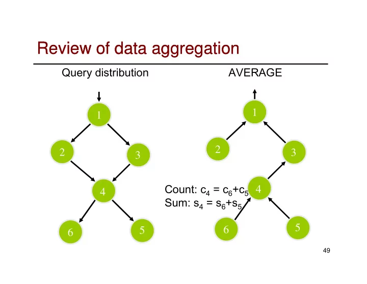
Review of data aggregation Review of data aggregation Query distribution AVERAGE 1 1 2 2 3 3 Count: c 4 = c 6 +c 5 4 4 Sum: s 4 = s 6 +s 5 5 6 5 6 49 nd problem: how to compute median? 1 nd problem: how to compute median? In a


slide-1
SLIDE 1

Review of data aggregation Review of data aggregation

AVERAGE 1 Query distribution 1

49

2 3 4 5 6 Count: c4 = c6+c5 Sum: s4 = s6+s5 2 3 4 5 6

slide-2
SLIDE 2

1nd

nd problem: how to compute median?

problem: how to compute median?

  • In a naïve way, the size of the message is

in the same order as # nodes in the subtree.

  • Last lecture: approximate median.

50

  • Last lecture: approximate median.
slide-3
SLIDE 3

2nd

nd problem: Aggregation tree in practice

problem: Aggregation tree in practice

  • Tree is a fragile structure.

– If a link fails, the data from the entire subtree is lost.

  • Fix #1: use multipath, a DAG instead of a

51

  • Fix #1: use multipath, a DAG instead of a

tree.

– Send 1/k data to each of the k upstream nodes (parents). – A link failure lost 1/k data

1 2 3 4 5 6 1 2 3 4 5 6

slide-4
SLIDE 4

Aggregation tree in practice Aggregation tree in practice

tree

52

tree DAG True value

slide-5
SLIDE 5

Fundamental problem Fundamental problem

  • Aggregation and routing are coupled
  • Improve routing robustness by multi-

path routing?

– Same data might be delivered multiple

53

– Same data might be delivered multiple times. – Problem: double-counting!

  • Decouple routing & aggregation

– Work on the robustness of each separately

1 2 3 4 5 6

slide-6
SLIDE 6

Order and duplicate insensitive (ODI) Order and duplicate insensitive (ODI) synopsis synopsis

  • Aggregated value is insensitive to the

sequence or duplication of input data.

  • Small-sizes digests such that any

particular sensor reading is accounted

54

particular sensor reading is accounted for only once.

– Example: MIN, MAX. – Challenge: how about COUNT, SUM?

slide-7
SLIDE 7

Aggregation framework Aggregation framework

  • Solution for robustness aggregation:

– Robust routing (e.g., multi-hop) + ODI synopsis.

  • Leaf nodes: Synopsis generation: SG(⋅).
  • Internal nodes: Synopsis fusion: SF(⋅) takes

55

  • Internal nodes: Synopsis fusion: SF(⋅) takes

two synopsis and generate a new synopsis of the union of input data.

  • Root node: Synopsis evaluation: SE(⋅)

translates the synopsis to the final answer.

slide-8
SLIDE 8

An easy example: ODI synopsis for An easy example: ODI synopsis for MAX/MIN MAX/MIN

  • Synopsis generation: SG(⋅).

– Output the value itself.

  • Synopsis fusion: SF(⋅)

– Take the MAX/MIN of the two 1 2 3

56

– Take the MAX/MIN of the two input values.

  • Synopsis evaluation: SE(⋅).

– Output the synopsis. 4 5 6

slide-9
SLIDE 9

Three questions Three questions

  • What do we mean by ODI, rigorously?
  • Robust routing + ODI
  • How to design ODI synopsis?

57

– COUNT – SUM – Sampling – Most popular k items – Set membership – Bloom filter

slide-10
SLIDE 10

Definition of ODI correctness Definition of ODI correctness

  • A synopsis diffusion algorithm is ODI-correct if

SF() and SG() are order and duplicate insensitive functions.

  • Or, if for any aggregation DAG, the resulting

synopsis is identical to the synopsis produced by

58

synopsis is identical to the synopsis produced by the canonical left-deep tree.

  • The final result is independent of the underlying

routing topology.

– Any evaluation order. – Any data duplication.

slide-11
SLIDE 11

Definition of ODI correctness Definition of ODI correctness

59

Connection to streaming model: data item comes 1 by 1.

slide-12
SLIDE 12

Test for ODI correctness Test for ODI correctness

1. SG() preserves duplicates: if two readings are duplicates (e.g., two nodes with same temperature readings), then the same synopsis is generated. 2. SF() is commutative. 3. SF() is associative.

60

3. SF() is associative. 4. SF() is same-synopsis idempotent, SF(s, s)=s. Theorem: The above properties are sufficient and necessary properties for ODI-correctness. Proof idea: transfer an aggregation DAG to a left-deep tree with the same output by using these properties.

slide-13
SLIDE 13

Proof of ODI correctness Proof of ODI correctness

1. Start from the DAG. Duplicate a node with out- degree k to k nodes, each with out degree 1. duplicates preserving.

61

slide-14
SLIDE 14

Proof of ODI correctness Proof of ODI correctness

2. Re-order the leaf nodes by the increasing value of the synopsis. Commutative.

62

slide-15
SLIDE 15

Proof of ODI correctness Proof of ODI correctness

3. Re-organize the tree s.t. adjacent leaves with the same value are input to a SF function. Associative.

SF

63

SF SG SF SG r1 SG SG r2 r2 r3

slide-16
SLIDE 16

Proof of ODI correctness Proof of ODI correctness

4. Replace SF(s, s) by s. same-synopsis idempotent.

SF SF SG SF SF SG

64

SF SG SF SG r1 SG SG r2 r2 r3 SF SG SG r1 SG r2 r3

slide-17
SLIDE 17

Proof of ODI correctness Proof of ODI correctness

5. Re-order the leaf nodes by the increasing canonical

  • rder. Commutative.

6. QED.

65

slide-18
SLIDE 18

Design ODI synopsis Design ODI synopsis

  • Recall that MAX/MIN are ODI.
  • Translate all the other aggregates

(COUNT, SUM, etc.) by using MAX.

  • Let’s first do COUNT.

66

  • Let’s first do COUNT.
  • Idea: use probabilistic counting.
  • Counting distinct element in a multi-set.

(Flajolet and Martin 1985).

slide-19
SLIDE 19

Counting distinct elements Counting distinct elements

  • Each sensor generates a sensor reading. Count the

total number of different readings.

  • Counting distinct element in a multi-set. (Flajolet

and Martin 1985).

  • Each element chooses a random number i ∈ [1, k].

67

  • Each element chooses a random number i ∈ [1, k].
  • Pr{CT(x)=i} = 2-i, for 1i k-1. Pr{CT(x)=k}= 2-(k-1).
  • Use a pseudo-random generator so that CT(x) is a

hash function (deterministic). 1

½ ¼ 1/8 1/16 …..

slide-20
SLIDE 20

Counting distinct elements Counting distinct elements

  • Synopsis: a bit vector of

length k>logn.

  • SG(): output a bit vector s
  • f length k with CT(k)’s bit

set.

  • SF(): bit-wise boolean OR

1 OR

68

  • SF(): bit-wise boolean OR
  • f input s and s’.
  • SE(): if i is the lowest

index that is still 0, output 2i-1/0.77351.

  • Intuition: i-th position will

be 1 if there are 2i nodes, each trying to set it with probability 1/2i 1 1 1 i=3

slide-21
SLIDE 21

Distinct value counter analysis Distinct value counter analysis

  • Lemma: For i<logn-2loglogn, FM[i]=1 with high

probability (asymptotically close to 1). For i ≥ 3/2logn+δ, with δ ≥ 0, FM[i]=0 with high probability.

  • The expected value of the first zero is

1

69

  • The expected value of the first zero is

log(0.7753n)+P(logn)+o(1), where P(u) is a periodic function of u with period 1 and amplitude bounded by 10-5.

  • The error bound (depending on variance) can be

improved by using multiple trials.

slide-22
SLIDE 22

Counting distinct elements Counting distinct elements

  • Check the ODI-correctness:

– Duplication: by the hash

  • function. The same reading x

generates the same value CT(x).

1 OR

70

CT(x). – Boolean OR is commutative, associative, same-synopsis idempotent.

  • Total storage: O(logn) bits.

1 1 1 i=3

slide-23
SLIDE 23

Robust routing + ODI Robust routing + ODI

  • Use Directed Acyclic Graph (DAG) to replace

tree.

  • Rings overlay:

– Query distribution: nodes in ring Rj are j hops from q.

71

– Query distribution: nodes in ring Rj are j hops from q. – Query aggregation: node in ring Rj wakes up in its allocated time slot and receives messages from nodes in Rj+1.

slide-24
SLIDE 24

Rings and adaptive rings Rings and adaptive rings

  • Adaptive rings: cope with network dynamics, node

deletions and insertions, etc.

  • Each node on ring j monitor the success rate of its

parents on ring j-1.

  • If the success rate is low, the node may change its

72

parent to other nodes with higher success rate.

  • Nodes at ring 1 may transmit multiple times to

ensure robustness.

slide-25
SLIDE 25

Implicit acknowledgement Implicit acknowledgement

  • Explicit acknowledgement:

– 3-way handshake. – Used for wired networks.

  • Implicit acknowledgement:

– Used on ad hoc wireless networks.

u v

73

– Node u sending to v snoops the subsequent broadcast from v to see if v indeed forwards the message for u. – Explores broadcast property, saves energy.

  • With aggregation this is problematic.

– Say u sends value x to v, and subsequently hears value z. – U does not know whether or not x is incorporated into z.

slide-26
SLIDE 26

Implicit acknowledgement Implicit acknowledgement

  • ODI-synopsis enables efficient implicit

acknowledgement.

– u sends to v synopsis x. – Afterwards u hears that v transmitting synopsis z. – u verifies whether SF(x, z)=z

74

– u verifies whether SF(x, z)=z u v

slide-27
SLIDE 27

Error of approximate answers Error of approximate answers

  • Two sources of errors:

– Algorithmic error: due to randomization and approximation. – Communication error: the fraction of sensor readings not accounted for in the final answer.

  • Algorithmic error depends on the choice of

75

  • Algorithmic error depends on the choice of

algorithm and is under control.

  • Communication error depends on the network

dynamics and robustness of routing algorithms.

slide-28
SLIDE 28

Simulation results Simulation results

76

Unaccounted node

slide-29
SLIDE 29

Simulation results Simulation results

77

Relative root mean square error

slide-30
SLIDE 30

More ODI synopsis More ODI synopsis

  • Distinct values
  • SUM
  • Second moment

78

  • Uniform sample
  • Most popular items
  • Set membership --- Bloom Filter
slide-31
SLIDE 31

Sum Sum

  • Naïve approach: for an item x with value c times,

make c distinct copies (x, j), j=1, …, c. Now use the distinct count algorithm.

  • When c is large, we set the bits as if we had

performed c successive insertions to the FM sketch.

  • First set the first δ = logc-loglogc bits to 1.

79

  • First set the first δ = logc-loglogc bits to 1.
  • Those who reached δ follow a binomial distribution:

each item reaches δ with prob 2-δ.

  • Explicitly insert those that reached bit δ by coin

flipping.

  • Powerful building block.
slide-32
SLIDE 32

Second moment Second moment

  • Kth moment µk=Σ xi

k, xi is the number of

sensor readings (frequency) of value i.

– µ0 is the number of distinct elements. – µ1 is the sum.

80

– µ2 is the square of L2 norm (variance, skewness

  • f the data).
  • The sketch algorithm for frequency

moments can be turned into an ODI easily by using ODI-sum.

The space complexity of approximating the frequency moments,

  • N. Alon, Y. Matias, and M. Szegedy. STOC 1996.
slide-33
SLIDE 33

Second moment Second moment

  • Random hash h( ): {0,1,…,N-1} {-1,1}
  • Define zi =h(i)
  • Maintain X = i xizi
  • E(X2) = E(i xizi)2 = E(i xi

2zi 2)+ E(i,jxixjzizj).

  • Choose the hash function to be pairwise

81

  • Choose the hash function to be pairwise

independent: Pr{h(i)=a,h(j)=b} = ¼.

  • E(zi

2)=1, E(zizj)= E(zi) E(zj)= 0.

  • Now E(X2) = i xi

2.

  • ODI: Each sensor of value i generates zi, then use

ODI-sum.

  • The final answer is X2
slide-34
SLIDE 34

More ODI synopsis More ODI synopsis

  • Distinct values
  • SUM
  • Second moment

82

  • Uniform sample
  • Most popular items
  • Set membership --- Bloom Filter
slide-35
SLIDE 35

Uniform sample Uniform sample

  • Each sensor has a reading. Compute a uniform

sample of a given size k.

  • Synopsis: a sample of k tuples.
  • SG(): output (value, r, id), where r is a uniform

random number in range [0, 1].

  • SF(): output the k tuples with the k largest r values.

83

  • SF(): output the k tuples with the k largest r values.

If there are less than k tuples in total, out them all.

  • SE(): output the values in s.
  • ODI-correctness is implied by “MAX” and union
  • peration in SF().
  • Correctness: the largest k random numbers is a

uniform k sample.

slide-36
SLIDE 36

Most popular items Most popular items

  • Return the k values that occur the most frequently

among all the sensor readings

  • Synopsis: a set of k most popular items.
  • SG(): output (value, weight) pair, with weight=CT(k),

k>logn.

  • SF(): for each distinct value v, discard all but the

84

  • SF(): for each distinct value v, discard all but the

pair with max weight. Then output the k pairs with max weight.

  • SE(): output the set of values.
  • Note: we attach a weight to estimate the frequency.
  • Many aggregates that can be approximated by

using random samples now have ODI-synopsis, e.g., median.

slide-37
SLIDE 37

Set membership: Bloom Filter Set membership: Bloom Filter

  • A compact data structure to encode set

containment.

  • Widely used in networking applications.

85

  • Given: n elements S={x1, x2, , xn}.
  • Answer query: whether x is in S?
  • Allow a small false positive (an element not in S

might be reported as “yes”).

slide-38
SLIDE 38

Bloom filter Bloom filter

  • An array of m bits.
  • Insert: for x 2 S, use k

random hash functions and set hj(x) to “1”.

86

set hj(x) to “1”.

  • Query: to check if y is in S,

search all buckets hj(y), if all “1”, answer “yes”.

  • No false negative. Small

false positive.

slide-39
SLIDE 39

Bloom filter tricks Bloom filter tricks

  • Union of S1 and S2:

– Take “OR” of their bloom filters. – ODI aggregation.

  • Shrink the size to half:

87

  • Shrink the size to half:

– OR the first and second halves.

slide-40
SLIDE 40

Counting bloom filter Counting bloom filter

  • Handle element insertion and deletion
  • Each bucket is a counter.
  • Insert: increase by “1” on the hashed

locations.

88

locations.

  • Delete: decrease by “1”.
  • Be careful about buffer overflow.
slide-41
SLIDE 41

Spectral bloom filter Spectral bloom filter

  • Record multi-set {x1, x2, , xn}, each item

xi has a frequency fi.

  • Insert: add fi to each bucket.
  • Retrieve: return the smallest bucket value

89

  • Retrieve: return the smallest bucket value

from the hashed locations.

  • Idea: the smallest bucket is unlikely to be

polluted.

slide-42
SLIDE 42

Bloom filter applications Bloom filter applications

  • Traditional applications:

– Dictionary, UNIX-spell checker.

  • Network applications:

– Cache summary in content delivery network.

90

– Cache summary in content delivery network. – Resource routing, etc. – Read the survey for more….

  • Good for sensor network setting:

– ODI, compact, many algebraic properties.

slide-43
SLIDE 43

Conclusion Conclusion

  • Due to the high dynamics in sensor networks,

robust aggregates that are insensitive to order and duplication are very attractive – they provide the flexibility of using any multi-path routing algorithms and re-transmission.

91

  • Use ODI-synopsis as black box operators to

replace naïve operators in more complex data structures.

slide-44
SLIDE 44

Is the problem solved? NO Is the problem solved? NO

  • Best effort multi-path routing does not guarantee

all data have been incorporated.

– Blackbox setting.

  • ODI synopsis translates everything to MAX,

92

which is not robust to outliers!

– Sensor malfunction. – Malicious attacks.

  • For exemplary aggregations (MAX, MIN), the

final result is a single sensor value, but all nodes are examined. – Can we improve?

slide-45
SLIDE 45

CountTorrent CountTorrent

  • To improve routing robustness, deliver

each value multiple times to make sure at least one copy arrives

– Synopsis diffusion: aggregation of the same

93

– Synopsis diffusion: aggregation of the same value for multiple times does not result in double counting. – CountTorrent: remember what value has been included in the aggregation in an implicit manner.

slide-46
SLIDE 46

How to record the members in the How to record the members in the aggregate? aggregate?

  • In the naive way, keep the members

explicitly.

– Storage cost /communication cost too high – It loses the point of aggregation.

94

– It loses the point of aggregation.

  • In the implicit way

– Label the aggregates

slide-47
SLIDE 47

CountTorrent CountTorrent

  • Each node has a label: a 0,1 string
  • Two nodes can have their data aggregated if

their labels are the same except the last bit.

  • After aggregation, remove the last bit and assign

95

  • After aggregation, remove the last bit and assign

the label to the aggregated data.

  • Gossip-style communication: each node

exchanges its value with neighbors.

slide-48
SLIDE 48

CountTorrent example CountTorrent example

  • For any 2 nodes, their labels are neither the same nor is

either one a substring of the other

  • All N labels can be merged pairwise and recursively to

yield , the empty string.

96

slide-49
SLIDE 49

Aggregation Aggregation

  • Each node keeps a buffer of received

value/label pair

  • Consolidate: try to merge the data in the buffer

97

slide-50
SLIDE 50

How to assign labels? How to assign labels?

  • Each node is given the label of a leaf

node.

98

slide-51
SLIDE 51

Conclusion Conclusion

  • Aggregation sometimes requires careful design

to tradeoff accuracy & storage/message size.

  • Aggregation incurs information loss, making

99

  • Aggregation incurs information loss, making

robust estimation more difficult. E.g. a single

  • utlier reading can screw up MAX/MIN

aggregates.