
SLIDE 1
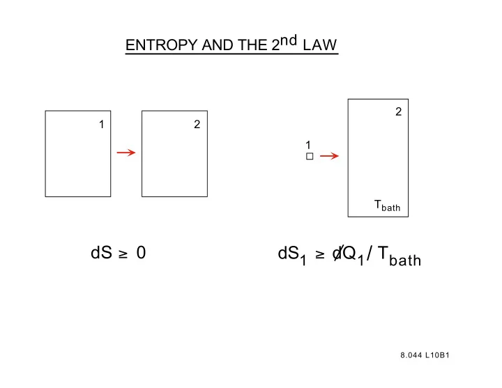
ENTROPY AND THE 2nd LAW
2 1 2 1 Tbath
dS ≥ 0 dS1 ≥ dQ1/ Tbath
8.044 L10B1
S as a State Function Note: adiabatic ( d /Q = 0) constant S if the - - PowerPoint PPT Presentation
ENTROPY AND THE 2nd LAW 2 1 2 1 T bath dS 1 dQ 1 / T bath dS 0 8.044 L10B1 S as a State Function Note: adiabatic ( d /Q = 0) constant S if the change is quasistatic. This is the origin of the sub- script S on the adiabatic
8.044 L10B1
8.044 L10B2
8.044 L10B3
8.044 L10B4
8.044 L10B5
8.044 L10B6
8.044 L10B7
8.044 L10B8
8.044 L10B9
8.044 L10B10
8.044 L10B11
8.044 L10B12
8.044 L10B13
8.044 L10B14
8.044 L10B15
MIT OpenCourseWare http://ocw.mit.edu
8.044 Statistical Physics I
Spring 2013 For information about citing these materials or our Terms of Use, visit: http://ocw.mit.edu/terms.