Small-scale galaxy dynamics: the pairwise velocity dispersion Jon - - PowerPoint PPT Presentation

small scale galaxy dynamics the pairwise velocity
SMART_READER_LITE
LIVE PREVIEW

Small-scale galaxy dynamics: the pairwise velocity dispersion Jon - - PowerPoint PPT Presentation

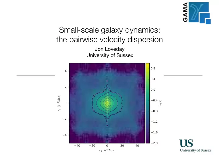
Small-scale galaxy dynamics: the pairwise velocity dispersion Jon Loveday University of Sussex Outline RSD overview Galaxy pairwise velocity dispersion (PVD) - why measure it? GAMA data and mocks Ways of measuring PVD Results:


slide-1
SLIDE 1

Small-scale galaxy dynamics: the pairwise velocity dispersion

Jon Loveday University of Sussex

slide-2
SLIDE 2

Outline

  • RSD overview
  • Galaxy pairwise velocity dispersion (PVD)
  • why measure it?
  • GAMA data and mocks
  • Ways of measuring PVD
  • Results: luminosity dependence
  • Future work
  • See Loveday+ 2018, MNRAS, 474, 3435

slide-3
SLIDE 3

Redshift-space distortions

  • Redshift space measurements are distorted by motions of galaxies relative to

Hubble Flow

  • Small scales: random motions → “Fingers of God”
  • Large scales: coherent bulk motions towards high-density regions →

growth factor

  • Pairwise velocity dispersion (PVD) σ12 is the dispersion in relative velocity

between pairs of galaxies as a function of projected separation

Mock: real space

slide-4
SLIDE 4

Redshift-space distortions

  • Redshift space measurements are distorted by motions of galaxies relative to

Hubble Flow

  • Small scales: random motions → “Fingers of God”
  • Large scales: coherent bulk motions towards high-density regions →

growth factor

  • Pairwise velocity dispersion (PVD) σ12 is the dispersion in relative velocity

between pairs of galaxies as a function of projected separation

Mock: redshift space

slide-5
SLIDE 5

Motivation - why measure PVD?

  • Originally used to estimate Ωm via

cosmic virial theorem (Peebles 1976)

  • First evidence for Ωm < 1
  • However, results are sensitive to

presence or absence of rich clusters (Mo+ 1993)

  • Quantify FoG effect
  • Needed to model linear infall
  • Constrain HOD models

(dependence on stellar mass and scale, e.g. Tinker+ 2007)

  • Clarify luminosity-dependence
  • Test modified gravity models

Li+ 2006, MNRAS, 368, 1

slide-6
SLIDE 6

Constraining modified gravity models

Hellwing+ 2014, PRL, 112, 221102

LOS Radial

slide-7
SLIDE 7

Galaxy and Mass Assembly (GAMA)

  • Three 12 x 5 deg equatorial fields to

r = 19.8: G09, G12, G15

  • Target density ∼1000/deg2
  • Fully automated redshifts
  • 183,010 galaxies with reliable

redshifts (98.5% completeness, inc high-density regions)

  • Mean redshift z̅ = 0.23
  • Derived parameters: stellar masses, 


groups, environment

  • Matched-aperture photometry

GALEX-SDSS-UKIDSS

  • Southern fields (G02, G23) less

complete

G09 G12 G15 G23

www.gama-survey.org

G02

slide-8
SLIDE 8

SDSS Main

slide-9
SLIDE 9

GAMA-II

slide-10
SLIDE 10

Spectroscopic completeness (eq regions)

Number Target completeness Redshift completeness (average) Liske+ 2015

slide-11
SLIDE 11

Redshift completeness maps

Liske+ 2015

slide-12
SLIDE 12

Mock comparison data

  • Good test of methods since peculiar velocities known for each galaxy
  • Main comparison/testbed:
  • Millennium-WMAP7 Simulation (Guo et al. 2013)
  • Gonzalez-Perez+ 2014 GALFORM model
  • GAMA-like lightcones from Merson et al. 2013
  • 26 realisations: plots show average and standard deviation
  • Use zcos and zobs to measure `true’ PVD
  • Compare with estimates using only observable information (RA, dec, zobs)
  • Also compare with EAGLE hydrodynamical simulation RefL0100N1504 


(Crain et al. 2015; Schaye et al. 2015; McAlpine et al. 2016)

slide-13
SLIDE 13
  • Two-point correlation function 


ξ(r⊥, r∥): excess probability of

  • bserving two galaxies separated by

distance r⊥ perpendicular to line of sight (LOS), r∥ parallel to LOS

  • Integrate along LOS to obtain 


projected correlation function wp(r⊥)

  • Invert to obtain real-space ξr(r)
  • PVD then determined via streaming
  • r dispersion models
  • First need to choose model for

pairwise velocity distribution function …

Galaxy clustering measurements

Loveday+ 2018

slide-14
SLIDE 14

Pairwise velocity distribution function

  • Determined via 2-d Fourier transform of ξ(r⊥, r∥) (Landy+ 1998, 2002)
  • Exponential function significantly better fit than Gaussian for both GAMA and

mocks, in line with previous work

GAMA GALFORM mocks exponential Gaussian Loveday+ 2018

slide-15
SLIDE 15

Method 1: Streaming model

  • Assumes model for mean streaming velocity (e.g. Peebles 1980, Davis &

Peebles 1983, Juszkiewicz+ 1999)

  • Predicted 2-d correlation function ξ(r⊥, r∥) given by convolving ξr(r) with f(v):

1 + ξ(r?, rk) = H0 Z 1

1

 1 + ξr ✓q r2

? + y2

◆ f(v)dy f(v) = 1 √ 2σ12 exp − √ 2|v − ¯ v| σ12 ! v ≡ H0(rk − y)

¯ v(r)

Juszkiewicz+ 1999

slide-16
SLIDE 16

Method 2: Dispersion model

  • Rather than assume mean streaming motion, convolve Kaiser linear infall model

with f(v) centred on zero (Peacock & Dodds 1994, Cole+ 1995)

  • Kaiser infall in configuration space given by spherical harmonics (Hamilton 1992):
  • Predicted 2-d clustering given by convolution of ξʹ with f(v):

Kaiser linear infall Small-scale dispersion

slide-17
SLIDE 17

Mock tests

  • Streaming model recovers true PVD well on very small scales (r ≲ 1 h−1 Mpc)
  • Dispersion model performs better on larger scales (r ≲ 10 h−1 Mpc)

Streaming model Dispersion model

Loveday+ 2018 ‘truth’

slide-18
SLIDE 18

Results: PVD luminosity dependence

  • GALFORM mocks consistent with

GAMA for luminous galaxies (Mr ≲ −20)

  • Mock PVDs systematically higher for

fainter galaxies

  • EAGLE simulations largely consistent

with GALFORM

Loveday+ 2018

slide-19
SLIDE 19

Summary

  • PVD measured to ~10 × smaller scales than previous work (e.g. Hawkins et al.

2003, Jing & Borner 2004, Li et al. 2006)

  • In agreement with previous work, we find that the pairwise velocity distribution

is much better fit by an exponential than a Gaussian function

  • The dispersion model can make reliable predictions of the PVD for projected

separations 0.01–10 h−1 Mpc

  • The PVD peaks at σ12 ≈ 600 km s−1 at projected separations r⊥ ≈ 0.3 h−1 Mpc
  • On small scales, r⊥ ≲ 1 h−1 Mpc, the measured PVD for GAMA galaxies

declines slightly from ≈ 600 km s−1 at high luminosities to ≈ 400 km s−1 at low luminosities

  • The GALFORM mocks do a good job at matching the observed PVD for

luminous galaxies, but overpredict the PVD for fainter objects.

slide-20
SLIDE 20

Future prospects

  • Greatest challenge for utilising PVD

measurements is accurate modelling on non-linear scales

  • Galaxy feedback processes, as well as

cosmology, will need to be taken into account

  • 4MOST WAVES:
  • Wide survey will observe ~ 1 million

galaxies to ~106 M☉ to z ≈ 0.2 over 1600 deg2

  • 4MOST/LSST cross-correlation

synergies?

https://wavesurvey.org SDSS main GAMA Wide Deep UltraDeep