Solution Recording and Playback: Vortex Shedding This tutorial - - PDF document

STAR-CCM+ User Guide 6663 Version 7.03.027

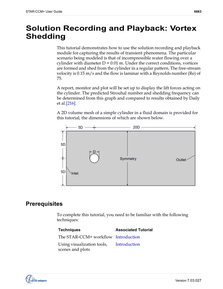
Solution Recording and Playback: Vortex Shedding

This tutorial demonstrates how to use the solution recording and playback module for capturing the results of transient phenomena. The particular scenario being modeled is that of incompressible water flowing over a cylinder with diameter D = 0.01 m. Under the correct conditions, vortices are formed and shed from the cylinder in a regular pattern. The free-stream velocity is 0.15 m/s and the flow is laminar with a Reynolds number (Re) of 75. A report, monitor and plot will be set up to display the lift forces acting on the cylinder. The predicted Strouhal number and shedding frequency can be determined from this graph and compared to results obtained by Daily et al.[216]. A 2D volume mesh of a simple cylinder in a fluid domain is provided for this tutorial, the dimensions of which are shown below.

Prerequisites

To complete this tutorial, you need to be familiar with the following techniques:

Techniques Associated Tutorial

The STAR-CCM+ workflow Introduction Using visualization tools, scenes and plots Introduction

STAR-CCM+ User Guide Solution Recording and Playback: Vortex Shedding 6664 Version 7.03.027

Importing the Mesh

• Start up STAR-CCM+ in a manner that is appropriate to your working

environment and create a New Simulation.

• Save the new simulation to disk with the file name

vortexShedding.sim

We will begin by importing the volume mesh.

• Select File > Import > Import Volume Mesh from the menu.

The Open dialog will appear.

• Navigate to the /doc/tutorials/simpleFlow subdirectory of your

STAR-CCM+ installation directory and select

vortexSheddingDomainMesh.ccm

A geometry scene is automatically created after the mesh has been successfully imported. The boundaries have been pre-defined, so no further action is required.

• Create a mesh scene and examine the 2D mesh.

Selecting Physics Models

A physics continuum was added to the object tree when the volume mesh was imported. We will select the physics models required to run this case.

STAR-CCM+ User Guide Solution Recording and Playback: Vortex Shedding 6665 Version 7.03.027

The fluid used in this tutorial is water, and the flow is incompressible and

• laminar. Vortex shedding is a periodic phenomenon and will require the

use of a transient solver.

• Rename the Continua > Physics 1 continuum to Fluid.
• Right-click on the Fluid > Models node and choose Select models...

The Fluid Model Selection dialog will guide you through the model selection

• process. Select the following models:
• Implicit Unsteady from the Time box.
• Liquid from the Material box.
• Coupled Flow from the Flow box.
• Constant Density from the Equation of State box.
• Laminar from the Viscous Regime box.
• Click Close.

The selected models are shown in the Fluid > Models node in the object tree.

Modifying Material Properties and Setting Initial Conditions

Modify the material properties of water, so that the correct Reynolds number is obtained.

• Within the Fluid continuum, select the Models > Liquid > H2O >

Material Properties > Density > Constant node and set its Value property to

STAR-CCM+ User Guide Solution Recording and Playback: Vortex Shedding 6666 Version 7.03.027

1 kg/m^3

• Select the Dynamic Viscosity > Constant node and set its Value property to

2.0E-5 Pa-s

Set the initial conditions so that the simulation will begin with the fluid in a state of motion.

• Select the Fluid > Initial Conditions > Velocity > Constant node. In the

Properties window, set the Value property to [0.15, 0.0, 0.0] m/s

Setting Boundary Conditions

Set the required velocity at the inlet boundary.

• Select the Regions > Fluid_Domain > Boundaries > Inlet >

Physics Conditions > Velocity Specification node. In the Properties window,

STAR-CCM+ User Guide Solution Recording and Playback: Vortex Shedding 6667 Version 7.03.027

set the Method property to Components.

• Select the Inlet > Physics Values > Velocity > Constant node and set its

Value property to [0.15, 0.0, 0.0] m/s

• Save the simulation

.

Creating a Scalar Scene

Create a scalar scene displaying vorticity. This will be used to visualize the solution while the simulation is running.

• Create a new scalar scene.
• Click on the scene/plot button located above the object tree.

STAR-CCM+ User Guide Solution Recording and Playback: Vortex Shedding 6668 Version 7.03.027

• Select the Displayers > Scalar 1 > Scalar Field node.
• In the Properties window set the Function property to Vorticity >

Magnitude.

• In the same window, set the following properties:
• Select the Displayers > Scalar 1 node. In the Properties window, set the

Contour Style property to Smooth Filled.

• Click on the simulation button to return to the STAR-CCM+ simulation
• bject tree.

We will add an annotation displaying solution time to the scene.

• Expand the Tools > Annotations node and drag the Solution Time node

Property Value

Min Max 28 Clip Off

STAR-CCM+ User Guide Solution Recording and Playback: Vortex Shedding 6669 Version 7.03.027

into the scene. The Solution Time annotation is added to the bottom left of the scene.

Preparing the Lift Plot

We will monitor the lift that the cylinder wall is experiencing. This will be used to determine the period of oscillation for the vortex shedding. First create a report:

• Right-click on the Reports node and select New Report > Force Coefficient.
• Rename the new plot to Coefficient of Lift.

In the Properties window of the Coefficient of Lift node, do the following:

• Set the Reference Velocity to 0.15 m/s
• Set the Reference Area to 0.01 m^2
• Set the Force Option to Pressure.
• Set the Direction to [0.0, 1.0, 0.0]
• Click to the right of the Parts property. In the object selection dialog, tick

STAR-CCM+ User Guide Solution Recording and Playback: Vortex Shedding 6670 Version 7.03.027

the checkbox next to Regions > Fluid_Domain > Cylinder. The completed Properties window is shown below. Create a monitor and plot from this report.

• Right-click on the Coefficient of Lift node and select

Create Monitor and Plot from Report.

STAR-CCM+ User Guide Solution Recording and Playback: Vortex Shedding 6671 Version 7.03.027

A new monitor and plot is added to the Monitors and Plots nodes respectively. We will now modify the monitor so that the data is plotted against time; the default setting would plot the data against iterations.

• Select the Monitors > Coefficient of Lift Monitor node. In the Properties

window, set the Trigger property to Time Step.

• Open the Coefficient of Lift Monitor Plot by right-clicking on its node in the
• bject tree and selecting Open.

Modifying Solver Settings

Modify the solver settings to more appropriate values for this case.

STAR-CCM+ User Guide Solution Recording and Playback: Vortex Shedding 6672 Version 7.03.027

• Select the Solvers > Implicit Unsteady node.
• In the Properties window, set the Time-Step to 0.02 s
• In the same window, set the Temporal Discretization to 2nd-order.
• Select the Solvers > Coupled Implicit node and set its Courant Number

property to 100

Setting Up Stopping Criteria

Reduce the number of inner iterations for each time step and extend the maximum time the solver will be allowed to run.

• Select the Stopping Criteria > Maximum Inner Iterations node and set its

Maximum Inner Iterations property to 15

• Select the Stopping Criteria > Maximum Physical Time node and set its

Maximum Physical Time property to 8 s

• Save the simulation

Setting Up the Solution History File

Create a new solution history (.simh) file and use it to store selected solution data at specified time intervals.

STAR-CCM+ User Guide Solution Recording and Playback: Vortex Shedding 6673 Version 7.03.027

• Right-click on the Solution Histories node and select New...

The Save dialog appears. Choose a location where you would like to store the solution history file.

• Enter vortexSheddingData.simh as the name of the solution history

file.

• Click Save.

STAR-CCM+ User Guide Solution Recording and Playback: Vortex Shedding 6674 Version 7.03.027

A new sub-node containing the name of the solution history file is added to the object tree below the Solution Histories node. The red asterisk next to this node means that data will be actively written to the file when the simulation runs. Choose what data to save to the solution history file. As this is a vortex shedding case it would be appropriate to store the results for pressure, velocity and vorticity.

• Select the Solution Histories > vortexSheddingData node. In the Properties

window, click on the (property customizer) button next to the

Scalar Functions property.

The Scalar Functions dialog appears.

• Use the > (Add selected) button to select the following items:
• Pressure
• Velocity

STAR-CCM+ User Guide Solution Recording and Playback: Vortex Shedding 6675 Version 7.03.027

• Vorticity

The selections are added to the right-hand side column, as shown below.

• Click OK to close the dialog.

Set the frequency with which the selected data will be written to the solution history file. We would like the data to be written every time step.

• Select the Solution Histories > vortexSheddingData > Update node and set

its Update Policy property to Time Step.

• Select the Update > Update Frequency node. In the Properties window,

STAR-CCM+ User Guide Solution Recording and Playback: Vortex Shedding 6676 Version 7.03.027

ensure that the Number of Time Steps property is set to 1

• Return to the Solution Histories > vortexSheddingData node. A summary
• f the properties for the solution history file is shown in the Properties

window. The Auto-record property will, when ticked, record the data to the solution history file at the required intervals. If you do not want to record the data when the solver is running, simply clear this checkbox. The Regions property is automatically populated with all regions in the simulation. In cases with multiple regions, you may remove regions by clicking to the right

• f the Regions property and clearing the checkbox next to the region you

want to remove. The Path property displays the relative path to the simulation history file. The States property displays the number of saved states stored in the selected solution history file; currently this is displaying 0 as the solver has not yet run.

• Save the simulation

.

Running the Simulation

The simulation is now ready to be run.

• Click on the

(Run) button. While the simulation is running you can click on the tabs at the top of the Graphics window to switch between the plot and the scene. The Residuals display will be created automatically and shows the progress of the solvers. The simulation will continue until the physical time of the simulation reaches 8 seconds. While the simulation is running, the Current Solution sub-node under the Solution View node displays the current Iteration,

Time Step, and Solution Time. The selected data is saved to the solution

history file at every time step.

• While the simulation is running, select the Scalar Scene 1 tab at the top
• f the Graphics window to visualize the solution.
• When the simulation has finished running, click on the

(Save) button.

STAR-CCM+ User Guide Solution Recording and Playback: Vortex Shedding 6677 Version 7.03.027

Visualizing the Results

The scalar scene after 8 s is shown below.

STAR-CCM+ User Guide Solution Recording and Playback: Vortex Shedding 6678 Version 7.03.027

The Coefficient of Lift monitor plot is shown below.

Validating the Results

From the scalar scene and the monitor plot, it is clear that vortex shedding is occurring. The Strouhal number (St) is commonly used when describing

• scillating flows and is defined as:

Where f is the frequency of vortex shedding, D is the cylinder diameter, and U is the free-stream velocity. In this case, the Strouhal number is given as 0.15 by Daily et al. [216]. The theoretical frequency of vortex shedding is therefore calculated as 2.25 Hz, which gives a period of 0.444 seconds. The predicted period of shedding can be obtained by zooming into the last two troughs of the monitor plot.

• Click on the

(Toggle Plot Zoom) button in the Plot toolbar.

St fD U

• =

STAR-CCM+ User Guide Solution Recording and Playback: Vortex Shedding 6679 Version 7.03.027

• Drag a box around the last two troughs on the plot, as shown below.

STAR-CCM+ User Guide Solution Recording and Playback: Vortex Shedding 6680 Version 7.03.027

The resulting plot is shown below.

• Click on the scene/plot button.
• Select the Coefficient of Lift Monitor Plot > Axes > X Axis > Grid node. In the

Properties window, set the Spacing property to 0.02

• Click on the simulation button.

STAR-CCM+ User Guide Solution Recording and Playback: Vortex Shedding 6681 Version 7.03.027

The enlarged scale on the X axis makes it possible to measure the period. The predicted period is shown to be approximately 0.44 seconds. Note that a relatively large time step was used for this tutorial resulting in a limited number of data points in the plot. If you want more accurate results and a smoother plot, the time step should be reduced. There is a difference of less than 1% between the predicted period and the reference period, which is good agreement for this case. The corresponding predicted frequency of 2.27 Hz is also in good agreement with the theoretical frequency of vortex shedding of 2.25 Hz.

Creating a Recorded Solution View

The solution history file contains all the data that was specified in the previous part of the tutorial. Solution views are used to interrogate this data and make it available for post-processing. Properties of the solution view set the point in the solution history at which data is read. Data is read into a separate representation linked to the solution view.

• Select the Solution Histories > vortexSheddingData node. The number of

STAR-CCM+ User Guide Solution Recording and Playback: Vortex Shedding 6682 Version 7.03.027

states stored in the solution history file is displayed next to the States property. 400 states are stored in the solution history file. We will create a solution view to access the states.

• Right-click on the Solution Histories > vortexSheddingData node and select

Create Recorded Solution View.

STAR-CCM+ User Guide Solution Recording and Playback: Vortex Shedding 6683 Version 7.03.027

A new sub-node, vortexSheddingData_View, is added to the Solution Views

• node. The properties of the solution view node control the data shown by

the representation associated with it. An additional representation linked to this view was added to the object tree under the Representations node. This representation stores solution data from the solution history file.

• Click on the Scalar Scene 1 tab in the Graphics window.
• Drag and drop the Solution Views > vortexSheddingData_View node onto a

STAR-CCM+ User Guide Solution Recording and Playback: Vortex Shedding 6684 Version 7.03.027

blank area in the scene window.

STAR-CCM+ User Guide Solution Recording and Playback: Vortex Shedding 6685 Version 7.03.027

The scene is shown below. This scene corresponds to the data stored in the solution history file for the first time step. We will now adjust the solution time to display the solution data at 1.3 seconds.

• Select the Solution Views > vortexSheddingData_View node. In the

Properties window, click to the right of the Solution Time property. A slider bar will appear. Here you can drag the slider to change the physical time of the solution being displayed in the scene.

STAR-CCM+ User Guide Solution Recording and Playback: Vortex Shedding 6686 Version 7.03.027

• Drag the slider so that the time is approximately 1.3 seconds.

The scene will update as shown below. Values can also be entered rather than using the slider.

• Click to the right of the Solution Time property and enter 3 s

STAR-CCM+ User Guide Solution Recording and Playback: Vortex Shedding 6687 Version 7.03.027

The updated scene is shown below. Restore the scene to use the most recent solution from the simulation file (stored on the volume mesh representation).

• Drag the Solution Views > Current Solution node into the scene as

previously described.

• Save the simulation

Creating an Animation from the Solution View

We will now create an animation that will show the development of vortex shedding from the start to a regular periodic state.

• Drag the recorded solution view, Solution Views >

vortexSheddingData_View, back into the scene.

• Select the Solution Views > vortexSheddingData_View > Animation node. In

the Properties window, set the Animation Mode property to Solution Time.

STAR-CCM+ User Guide Solution Recording and Playback: Vortex Shedding 6688 Version 7.03.027

A new node, Solution Time Animation, will appear below the Animation node. When creating an animation, it is important to set the correct framerate. If the framerate is set too high, the video may reuse identical frames. If the framerate is set too low, the video may appear to play too quickly. One way to determine the correct framerate is to divide the total number of states (frames) by the total physical time of the simulation. In this case we have 400 states and a physical time of 8 seconds. Knowing this, we can calculate that 50 frames make up one second of simulation time. We will now adjust the framerate for the animation.

• Click on the scene/plot button.
• Select the Scalar Scene 1 > Attributes > Animation node. In the Properties

window, set the Target frame rate (fps) property to 50 We will now record the animation.

• Click on the

(Write Movie) button in the Animation toolbar. The Write animation dialog appears.

• Set the Animation Length to 8
• Set the Size to a resolution of your choice.
• Set the File Name to vorticityAnimation.avi.

STAR-CCM+ User Guide Solution Recording and Playback: Vortex Shedding 6689 Version 7.03.027

The completed dialog is shown below.

• Click Save to write the animation to disk.
• Play back the animation using a player of your choice.

Summary

This tutorial covered the following:

• Creating a Solution History file.
• Selecting appropriate scalars to save to the Solution History file at

suitable intervals.

• Plotting the lift coefficient and validating the period of shedding against

reference data.

• Creating a Recorded Solution View.
• Viewing recorded solution data in a scene.
• Recording an animation from the Solution History file.

Bibliography

[216] Daily, J.W., and Harleman, D.R.F. Fluid Dynamics, Addison-Wesley, MA, 1966