Spectral Clustering Spectral Clustering? Spectral methods Methods - - PowerPoint PPT Presentation

spectral clustering
SMART_READER_LITE
LIVE PREVIEW

Spectral Clustering Spectral Clustering? Spectral methods Methods - - PowerPoint PPT Presentation

Spectral Clustering Spectral Clustering? Spectral methods Methods using eigenvectors of some matrices Involve eigen-decomposition (or spectral decomposition) Seungjin Choi Spectral clustering methods: Algorithms that cluster data


slide-1
SLIDE 1

Spectral Clustering

Seungjin Choi Department of Computer Science POSTECH, Korea seungjin@postech.ac.kr 1

Spectral Clustering?

  • Spectral methods

– Methods using eigenvectors of some matrices – Involve eigen-decomposition (or spectral decomposition)

  • Spectral clustering methods: Algorithms that cluster data points

using eigenvectors of matrices derived from the data

  • Closely related to spectral graph partitioning
  • Pairwise (Similarity-based) clustering methods

– Standard statistical clustering methods assume a probabilistic model that generates the observed data points – Pairwise clustering methods define a similarity function between pairs of data points and then formulates a criterion that the clustering must optimize 2

Spectral Clustering Algorithm: Bipartioning

  • 1. Construct affinity matrix

Wij =

  • exp{−βvi − vj2}

if i = j if i = j

  • 2. Calculate the graph Laplacian L:

L = D − W where D = diag{d1, . . . , dn} and di =

j Wij.

  • 3. Compute the second smallest eigenvector of the graph Laplacian

(denoted by u = [u1 · · · un]⊤, Fiedler vector)

  • 4. Partition ui’s by a pre-specified threshold value and assign data

points vi to cluster. 3
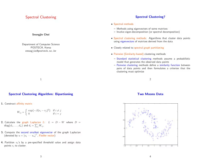
Two Moons Data

−1.5 −1 −0.5 0.5 1 1.5 2 2.5 3 −1 −0.5 0.5 1 1.5

4

slide-2
SLIDE 2

Two Moons Data: k-Means

−1.5 −1 −0.5 0.5 1 1.5 2 2.5 3 −0.8 −0.6 −0.4 −0.2 0.2 0.4 0.6 0.8 1 1.2

5

Two Moons Data: Fiedler Vector

20 40 60 80 100 120 140 160 180 200 −0.1 −0.08 −0.06 −0.04 −0.02 0.02 0.04 0.06

6

Two Moons Data: Spectral Clustering

−1.5 −1 −0.5 0.5 1 1.5 2 2.5 3 −0.8 −0.6 −0.4 −0.2 0.2 0.4 0.6 0.8 1 1.2

7

Graphs

  • Consider a connected graph G(V, E) where V = {v1, . . . , vn} and E

denote a set of vertices and a set of edges, respectively, with pairwise similarity values being assigned as edge weights.

  • Adjacency matrix (similarity, proximity, affinity matrix):

W = [Wij] ∈ Rn×n.

  • Degree of nodes: di =

j Wij.

  • Volume: vol(S1) = dS1 =

i∈S1 di.

8

slide-3
SLIDE 3

Neighborhood Graphs

Gaussian similarity function is given by w(vi, vj) = Wij = exp

  • −vi − vj2

2σ2

  • .
  • ǫ-neighborhood graph
  • k-nearest neighbor graph

9

Graph Laplacian

(Unnormalized) graph Laplacian is defined as L = D − W.

  • 1. For every vector x ∈ Rn, we have

x⊤Lx = 1 2

n

  • i=1

n

  • j=1

Wij(xi − xj)2 ≥ 0. (positive semidefinite)

  • 2. The smallest eigenvalue of L is 0 and the corresponding eigenvector

is 1 = [1 · · · 1]⊤, since D1 = W1, i.e, L1 = 0.

  • 3. L has n nonnegative eigenvalues, λ1 ≥ λ2 ≥ · · · ≥ λn = 0.

10 x⊤Lx = x⊤Dx − x⊤Wx =

n

  • i=1

dix2

i − n

  • i=1

n

  • j=1

Wijxixj = 1 2  

i

dix2

i − 2

  • i
  • j

Wijxixj +

  • j

djx2

j

  = 1 2

  • i
  • j

Wij(xi − xj)2. 11

Normalized Graph Laplacian

Two different normalization methods are popular, including:

  • Symmetric normalization:

Ls = D−1

2LD−1 2 = I − D−1 2WD−1 2.

  • Normalization related to random walks:

Lrw = D−1L = I − D−1W. 12

slide-4
SLIDE 4
  • 1. For every vector x ∈ Rn, we have

x⊤Lsx = 1 2

n

  • i=1

n

  • j=1

Wij

  • xi

√di − xj

  • dj

2 .

  • 2. Lsym and Lrw are positive semidefinite and have n nonnegative

real-valued eigenvalues, λ1 ≥ · · · λn = 0.

  • 3. λ is an eigenvalue of Lrw with eigenvector u if and only if λ is an

eigenvalue of Ls with eigenvector D1/2u.

  • 4. λ is an eigenvalue of Lrw with eigenvector u if and only if λ and u

solves the generalized eigenvalue problem Lu = λDu.

  • 5. 0 is an eigenvalue of Lrw with the constant one vector 1 as
  • eigenvector. 0 is an eigenvalue of Ls with eigenvector D1/21.

13

Unnormalized Spectral Clustering

  • 1. Construct a neighborhood graph with corresponding adjacency

matrix W.

  • 2. Compute the unnormalized graph Laplacian L = D − W.
  • 3. Find the k smallest eigenvectors of L and form the matrix U =

[u1 · · · uk] ∈ Rn×k.

  • 4. Treating each row of U as a point in Rk, cluster them into k groups

using k-means algorithm.

  • 5. Assign vi to cluster j if and only if row i of U is assigned to cluster

j. 14

Normalized Spectral Clustering: Shi-Malik

  • 1. Construct a neighborhood graph with corresponding adjacency

matrix W.

  • 2. Compute the unnormalized graph Laplacian L = D − W.
  • 3. Find the k smallest generalized eigenvectors u1, . . . , uk of the problem

Lu = λDu and form the matrix U = [u1 · · · uk] ∈ Rn×k.

  • 4. Treating each row of U as a point in Rk, cluster them into k groups

using k-means algorithm.

  • 5. Assign vi to cluster j if and only if row i of U is assigned to cluster

j. 15

Normalized Spectral Clustering: Ng-Jordan-Weiss

  • 1. Construct a neighborhood graph with corresponding adjacency

matrix W.

  • 2. Compute the normalized graph Laplacian Ls = D−1/2LD−1/2.
  • 3. Find the k smallest eigenvectors u1, . . . , uk of Ls and form the

matrix U = [u1 · · · uk] ∈ Rn×k.

  • 4. Form the matrix

U from U by re-normalizing each row of U to have unit norm, i.e., Uij = Uij/(

j Uij)1/2.

  • 5. Treating each row of

U as a point in Rk, cluster them into k groups using k-means algorithm.

  • 6. Assign vi to cluster j if and only if row i of

U is assigned to cluster j. 16

slide-5
SLIDE 5

Where does this spectral clustering algorithm come from?

  • Spectral graph partitioning
  • Properties of block (diagonal) matrix
  • Markov random walk

17

Pictorial Illustration of Graph Partitioning

18

Graph Partitioning: Bipartitioning

  • Consider a connected graph G(V, E) where V = {v1, . . . , vn} and E

denote a set of vertices and a set of edges, respectively, with pairwise similarity values being assigned as edge weights.

  • Graph bipartitioning involves taking the set V apart into two coherent

groups, S1 and S2, satisfying V = S1∪S2, (|V| = n), and S1∩S2 = ∅, by simply cutting edges connecting the two parts

  • Adjacency matrix (similarity, proximity, affinity matrix):

W = [Wij] ∈ Rn×n.

  • Degree of nodes: di =

j Wij.

  • Volume: vol(S1) = dS1 =

i∈S1 di.

19

Pictorial Illustration: Cut and Volume

  • cut(S1,S2)

=

  • vol(S1)

+

  • vol(S2)

  • S1 only

  • S2 only

20

slide-6
SLIDE 6

Graph Partitioning

The task is to find k disjoint sets, S1, . . . , Sk, given G = (V, E), where S1 ∩· · ·∩Sk = φ and S1 ∪· · ·∪Sk = V such that a certain cut criterion is minimized.

  • 1. Bipartitioning: cut(S1, S2) =

i∈S1

  • j∈S2 Wij.
  • 2. Multiway partitioning: cut(S1, . . . , Sk) = k

i=1 cut(Si, Si).

  • 3. Ratio cut: Rcut(S1, . . . , Sk) = k

i=1 cut(Si,Si) |Si|

.

  • 4. Normalized cut: Ncut(S1, . . . , Sk) = k

i=1 cut(Si,Si)

vol(Si) . 21

Cut: Bipartitioning

The degree of dissimilarity between S1 and S2 can be computed by the total weights

  • f edges that have been removed.

Cut(S1, S2) = X

i∈S1

X

j∈S2

Wij = 1 2 8 < : X

i∈S1

di + X

j∈S2

dj − X

i∈S1

X

j∈S1

Wij − X

i∈S2

X

j∈S2

Wij 9 = ; = 1 4 n (q1 − q2)⊤ L (q1 − q2)

  • ,

where qj = [q1j · · · qnj]⊤ ∈ Rn is the indicator vector which represents partitions, qij =  1, if i ∈ Sj 0, if i / ∈ Sj , for i = 1, . . . , n and j = 1, 2. Note that q1 and q2 are orthogonal, i.e., q⊤

1 q2 = 0.

22 Introducing bipolar indicator vector, x = q1 − q2 ∈ {+1, −1}n, the cut criterion is simplified as Cut(S1, S2) = 1 4x⊤Lx. The balanced cut involves the following combinatorial optimization problem arg min

x

x⊤Lx subject to 1⊤x = 0, x ∈ {1, −1}. Dropping the integer constrains (spectral relaxation), leads to the symmetric eigenvalue problem. The second smallest eigenvector of L corresponds to the solution, since the smallest eigenvalue of L is 0 and its associated eigenvector is 1. The second smallest eigenvector is known as Fiedler vector. 23

Rcut and Unnormalized Spectral Clustering: k = 2

Define the indicator vector x = [x1 · · · xn]⊤ with entries xi =   

  • |S|/|S|

if vi ∈ S −

  • |S|/|S|

if vi ∈ S. Then one can easily see that x⊤Lx = 2|V|Rcut(S, S), x⊤1 = 0, x = √n. 24

slide-7
SLIDE 7

arg min

S⊂V

Rcut(S, S) ≡ arg min

S⊂V

x⊤Lx, subject to x⊤1 = 0, xi is defined in previous slide, x = √n. The relaxation by discarding the condition on the discrete values on xi and instead allowing xi ∈ R, leads to arg min

x∈Rn

x⊤Lx, subject to x⊤1 = 0 and x = √n. The eigenvector associated with the second smallest eigenvalue of L. Rounding the eigenvector gives an approximate solution to the ratio cut problem. 25

Rcut and Unnormalized Spectral Clustering: k > 2

Define the indicator matrix X = [x1 · · · xk] ∈ Rn×k and xi = [x1,i · · · xn,i]⊤ ∈ Rn with entries xi,j =

  • 1/
  • |Sj|

if vi ∈ Sj if vi ∈ Sj. Then we have x⊤

i Lxi = 2cut(Si, Si)

|Si| , X⊤X = I. Rcut(S1, . . . , Sk) = 1 2

k

  • i=1

x⊤

i Lxi = 1

2tr

  • X⊤LX
  • .

26 arg min

S1,...,Sk

Rcut(S1, . . . , Sk) ≡ arg min

S1,...,Sk

tr

  • X⊤LX
  • ,

subject to X⊤X = I, Xis defined in previous slide. Then the relaxed problem becomes arg min

X∈Rn×k tr

  • X⊤LX
  • subject to X⊤X = I.

We determine the k smallest eigenvectors of L to form U and run k-means algorithm on the rows of U. 27

Ncut and Normalized Spectral Clustering: k = 2

Define the indicator vector x = [x1 · · · xn]⊤ with entries xi =   

  • vol(S)/vol(S)

if vi ∈ S −

  • vol(S)/vol(S)

if vi ∈ S. Then one can easily see that x⊤Lx = 2|V|Ncut(S, S), (Dx)⊤1 = 0, x⊤Dx = vol(V). 28

slide-8
SLIDE 8

arg min

S⊂V

Ncut(S, S) ≡ arg min

S⊂V

x⊤Lx, subject to (Dx)⊤1 = 0, xi is defined in previous slide, x⊤Dx = vol(V). Relaxing the problem gives arg min

x∈Rn

x⊤Lx, subject to (Dx)⊤1 = 0 and x⊤Dx = vol(V). Define y = D1/2x, then the problem is arg min

y∈Rn

y⊤ D−1/2LD−1/2

  • Ls

y, subject to y⊤D1/21 = 0 and y2 = vol(V). The solution y is given by the 2nd smallest eigenvector of Ls, implying that x is the 2nd smallest eigenvector of Lrw or equivalently the 2nd smallest generalized eigenvector of Lu = λDu. 29

Ncut and Normalized Spectral Clustering: k > 2

Define the indicator matrix X = [x1 · · · xk] ∈ Rn×k and xi = [x1,i · · · xn,i]⊤ ∈ Rn with entries xi,j =

  • 1/
  • vol(Sj)

if vi ∈ Sj if vi ∈ Sj. Then we have x⊤

i Lxi = 2cut(Si, Si)

vol(Si) , X⊤X = I, x⊤

i Dxi = 1,

Ncut(S1, . . . , Sk) = 1 2

k

  • i=1

x⊤

i Lxi = 1

2tr

  • X⊤LX
  • .

30 arg min

S1,...,Sk

Ncut(S1, . . . , Sk) ≡ arg min

S1,...,Sk

tr

  • X⊤LX
  • ,

subject to X⊤DX = I, Xis defined in previous slide. Then the relaxed problem becomes arg min

Y ∈Rn×k tr

  • Y ⊤D−1/2LD−1/2Y
  • subject to Y ⊤Y = I.

We determine the k smallest eigenvectors of Ls to form U and run k-means algorithm on the rows of U. 31

Markov Random Walk View of Normalized Cut

  • Melia and Shi 2001
  • Probabilistic interpretation of normalized cut
  • Data points are clustered on the basis of the eigenvectors of the

resulting transition probability matrix (constructed by the weights) 32

slide-9
SLIDE 9

Transition Probability Matrix

  • We define a Markov random walk over the graph by constructing a

transition probability matrix from the edge weights Pij = Wij

  • j Wij

, where

j Pij = 1 for all i.

  • The random walk proceeds by successively selecting points according

to j ∼ Pij where i specifies the current location.

  • If the graph is connected and non-bipartite (ergodic Markov

chain), then the random walk always possesses a unique stationary distribution π = [π1 · · · πn]⊤ such that π⊤P = π⊤, which is given by πi = di/vol(G). 33

Ncut via Transition Probabilities

Define P(S | S) = P(Xt+1 ∈ S | Xt ∈ S) where Xt is a state of Markov random walk model at time t. The Ncut and Markov random walk model has the following relation: Ncut(S, S) = P(S|S) + P(S|S). The minimization of Ncut actually seeks a cut through the graph such that a random walk seldom transitions from S to S or vice versa. 34

Random Walk: Properties

If we start from i0, the distribution of points it that we end up with after t steps, is given by i1 ∼ Pi0i1, i2 ∼ X

i1

Pi0i1Pi1i2 = h P 2i

i0i2

, i3 ∼ X

i1

X

i2

Pi0i1Pi1i2Pi2i3 = h P 3i

i0i3

, . . . it ∼ h P ti

i0it

, where P t = P P · · · P and [·]ij denotes the i, j component of the matrix. The distribution of points that we end up with in after t random steps converges as t increases.

35

Stochastic Matrix

The stochastic matrix P is defined by P = D−1W . To find out how P t behaves for large t, it is useful to examine the eigen-decomposition of the following symmetric matrix D−1

2W D−1 2 = λ1u1u⊤ 1 + λ2u2u⊤ 2 + · · · + λnunu⊤ n .

The symmetric matrix is related to P t since “ D−1

2W D−1 2

” · · · “ D−1

2W D−1 2

” = D

1 2 (P · · · P ) D−1 2.

This allows us to write the t step transition probability matrix in terms of the eigenvalues/vectors of the symmetric matrix P t = D−1

2

“ D−1

2W D−1 2

”t D

1 2

= D−1

2

“ λt

1u1u⊤ 1 + λt 2u2u⊤ 2 + · · · + λt nunu⊤ n

” D

1 2,

where λ1 = 1 and P ∞ = D−1

2 `u1u⊤ 1

´ D

1 2.

36

slide-10
SLIDE 10

Spectral Clustering: Stochastic Matrix

  • We are interested in the largest correction to the asymptotic limit

P t ≈ P ∞ + D−1

2

λt

2u2u⊤ 2

  • D

1 2.

  • Note that
  • u2u⊤

2

  • ij = ui2uj2 and thus the largest correction term

increases the probability of transitions between points that share the same sign of ui2 and decreases transitions across points with different signs.

  • Binary spectral clustering: Divide the points into clusters based on

the sign of the elements of u2 uj2 > 0 ⇒ cluster 1, otherwise cluster 0. 37

Equivalence

Proposition 1. If λ, x are solutions of Px = λx and P = D−1W, then (1 − λ), x are solutions of Lx = λDx . This proposition shows the equivalence between the spectral clustering formulated by the normalized cut and the eigenvalue/vectors of the stochastic matrix P. The largest eigenvector of P is 1 containing no information. The second smallest eigenvector in the normalized cut, corresponds to the second largest eigenvector of the stochastic matrix. 38

Suggested Further Readings

  • 1. P. K. Chan, M. D. F. Schlag, and J. Y. Zien, ”Spectral k-way ratio-cut partitioning

and clustering,” IEEE Trans. CAD of Integrated Circuits and Systems, 1994.

  • 2. J. Shi and J. Malik, ”Normalized cuts and image segmentation,” CVPR-1997.
  • 3. Y. Weiss, ”Segmentation using eigenvectors: A unifying view,” ICCV-1999.
  • 4. M. Meila and J. Shi, ”A random walks view of spectral segmentation,” AISTATS-

2001.

  • 5. C. Ding et al., ”A min-max cut algorithm for graph partitioning and data

clustering,” ICDM-2001.

  • 6. A. Ng, M. Jordan, and Y. Weiss, ”On spectral clustering:

Analysis and an algorithm,” NIPS-2001.

  • 7. U. von Luxburg, ”A tutorial on spectral clustering,” MPI for Biological Cybernetics,

TR-149, 2006.

39