
SLIDE 1
Structure from Motion
Computer Vision Jia-Bin Huang, Virginia Tech
Many slides from S. Seitz, N Snavely, and D. Hoiem
Structure from Motion Computer Vision Jia-Bin Huang, Virginia Tech - - PowerPoint PPT Presentation
Structure from Motion Computer Vision Jia-Bin Huang, Virginia Tech Many slides from S. Seitz, N Snavely, and D. Hoiem Administrative stuffs HW 3 due 11:55 PM, Oct 17 (Wed) Submit your alignment results! [Link] HW 2 will be out this
Computer Vision Jia-Bin Huang, Virginia Tech
Many slides from S. Seitz, N Snavely, and D. Hoiem
enforce rank 2 using SVD
image
(the intersection of the cameras’ baseline with the image plane
image to a line in the other
by SVD
Assume we have matched points x x’ with outliers
Tx x ~ x T x ~
T F T F ~
T
~ det F
Fx x T
http://www.3dcadbrowser.com/download.aspx?3dmodel=40454
Guidi et al. High-accuracy 3D modeling of cultural heritage, 2004
https://www.youtube.com/watch?v=1HhOmF22oYA
https://www.youtube.com/watch?v=bK6vCPcFkfk
Images Points: Structure from Motion Points More points: Multiple View Stereo Points Meshes: Model Fitting Meshes Models: Texture Mapping Images Models: Image-based Modeling
Slide credit: J. Xiao
Images Points: Structure from Motion Points More points: Multiple View Stereo Points Meshes: Model Fitting Meshes Models: Texture Mapping Images Models: Image-based Modeling
Slide credit: J. Xiao
Images Points: Structure from Motion Points More points: Multiple View Stereo Points Meshes: Model Fitting Meshes Models: Texture Mapping Images Models: Image-based Modeling
Slide credit: J. Xiao
Images Points: Structure from Motion Points More points: Multiple View Stereo Points Meshes: Model Fitting Meshes Models: Texture Mapping Images Models: Image-based Modeling
Slide credit: J. Xiao
Images Points: Structure from Motion Points More points: Multiple View Stereo Points Meshes: Model Fitting Meshes Models: Texture Mapping Images Models: Image-based Modeling
Slide credit: J. Xiao
Images Points: Structure from Motion Points More points: Multiple View Stereo Points Meshes: Model Fitting Meshes Models: Texture Mapping Images Models: Image-based Modeling
Example: https://photosynth.net/
Slide credit: J. Xiao
C’x’ will not exactly intersect
A least squares solution to a system of equations
X
x x'
X P x PX x AX
T T T T T T T T
v u v u
2 3 1 3 2 3 1 3
p p p p p p p p A
Further reading: HZ p. 312-313
1 v u w x 1 v u w x
T T T 3 2 1
p p p P
T T T 3 2 1
p p p P
𝐲 = 𝑥 𝑣 𝑤 1 = 𝑸𝒀 = 𝒒𝟐
𝑼
𝒒𝟑
𝑼
𝒒𝟒
𝑼
𝒀 = 𝒒𝟐
𝑼𝒀
𝒒𝟑
𝑼𝒀
𝒒𝟒
𝑼𝒀
𝑥 𝑣 𝑤 1 = 𝑣𝒒𝟒
𝑼𝒀
𝑤𝒒𝟒
𝑼𝒀
𝒒𝟒
𝑼𝒀
= 𝒒𝟐
𝑼𝒀
𝒒𝟑
𝑼𝒀
𝒒𝟒
𝑼𝒀
𝑣𝒒𝟒
𝑼𝒀 − 𝒒𝟐 𝑼𝒀
= 𝑣𝒒𝟒
𝑼 − 𝒒𝟐 𝑼 𝒀 = 𝟏
𝑤𝒒𝟒
𝑼𝒀 − 𝒒𝟑 𝑼𝒀
= 𝑤𝒒𝟒
𝑼 − 𝒒𝟑 𝑼 𝒀 = 𝟏
𝑣′𝒒′𝟒
𝑼𝒀 − 𝒒′𝟐 𝑼𝒀 = 𝑣′𝒒′𝟒 𝑼 − 𝒒′𝟐 𝑼 𝒀 = 𝟏
𝑤′𝒒′𝟒
𝑼𝒀 − 𝒒′𝟑 𝑼𝒀 = 𝑤′𝒒′𝟒 𝑼 − 𝒒′𝟑 𝑼 𝒀 = 𝟏
X P x PX x
matrices
4. X = V(:, end) Pros and Cons
corresponding images
1 v u w x 1 v u w x
T T T 3 2 1
p p p P
T T T T T T T T
v u v u
2 3 1 3 2 3 1 3
p p p p p p p p A
T T T 3 2 1
p p p P
Code: http://www.robots.ox.ac.uk/~vgg/hzbook/code/vgg_multiview/vgg_X_from_xP_lin.m
Figure source: Robertson and Cipolla (Chpt 13 of Practical Image Processing and Computer Vision)
ෝ 𝒚′ 𝒚′ 𝒚 ෝ 𝒚
𝑑𝑝𝑡𝑢 𝒀 = 𝑒𝑗𝑡𝑢 𝒚, ෝ 𝒚 2 + 𝑒𝑗𝑡𝑢 𝒚′, ෝ 𝒚′ 2
ෝ 𝒚′𝑈𝑮ෝ 𝒚=0
Further reading: HZ p. 318
ෝ 𝒚′𝑈𝑮ෝ 𝒚=0
𝑑𝑝𝑡𝑢 𝒀 = 𝑒𝑗𝑡𝑢 𝒚, ෝ 𝒚 2 + 𝑒𝑗𝑡𝑢 𝒚′, ෝ 𝒚′ 2
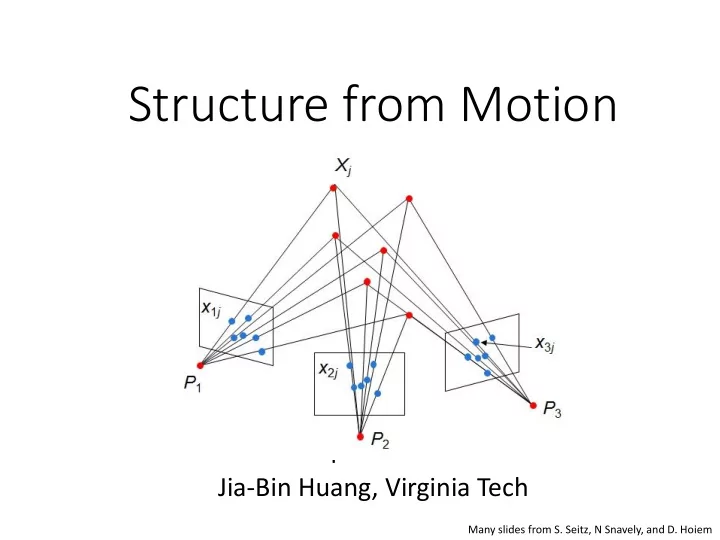
xij = Pi Xj , i = 1,… , m, j = 1, … , n
points Xj from the mn corresponding 2D points xij
x1j x2j x3j Xj P1 P2 P3 Slides from Lana Lazebnik
from the known mn corresponding points xij
be recovered up to a 4x4 projective transformation Q:
2mn >= 11m + 3n – 15
DoF in Pi DoF in Xj Up to 4x4 projective tform Q
two images using fundamental matrix
camera using all the known 3D points that are visible in its image – calibration/resectioning
cameras points
using fundamental matrix
camera using all the known 3D points that are visible in its image – calibration
compute new 3D points, re-optimize existing points that are also seen by this camera – triangulation
cameras points
using fundamental matrix
camera using all the known 3D points that are visible in its image – calibration
compute new 3D points, re-
seen by this camera – triangulation
adjustment cameras points
2 1 1
m i n j j i ij
x1j x2j x3j Xj P1 P2 P3 P1Xj P2Xj P3Xj
The Levenberg–Marquardt algorithm
The Ceres-Solver from Google
parameters directly from uncalibrated images
moving camera has a fixed intrinsic matrix
projective transformation matrix Q such that all camera matrices are in the form Pi = K [Ri | ti]
matrix, such as zero skew
pixel
adding points
similarity transform
subgraphs
Reconstruction of Cornell (Crandall et al. ECCV 2011) (best method with software available; also has good overview of recent methods)
Building Rome in a Day: Agarwal et al. 2009
Structure from motion under orthographic projection
3D Reconstruction of a Rotating Ping-Pong Ball
A factorization method. IJCV, 9(2):137-154, November 1992.
x X a1 a2
homogeneous coordinates
1. We are given corresponding 2D points (x) in several frames 2. We want to estimate the 3D points (X) and the affine parameters of each camera (A)
x X a1 a2
t AX x
y x
t t Z Y X a a a a a a y x
23 22 21 13 12 11
Projection of world origin
n k ik ij ij
n
1
1 ˆ x x x
i i i
t X A x
j i n k k j i n k i k i i j i n k ik ij
n n n X A X X A t X A t X A x x ˆ 1 1 1
1 1 1
j i ij
X A x ˆ ˆ
2d normalized point (observed) 3d normalized point Linear (affine) mapping
mn m m n n n m
2 1 2 22 21 1 12 11 2 1 2 1
Camera Parameters (2mx3) 3D Points (3xn) 2D Image Points (2mxn)
Can we recover the camera parameters and 3d points?
cameras (2m) points (n)
n m mn m m n n
2 1 2 1 2 1 2 22 21 1 12 11
Source: M. Hebert
Source: M. Hebert
Source: M. Hebert
Source: M. Hebert
Source: M. Hebert
A ~ X ~
We get the same D by using any 3×3 matrix C and applying the transformations A → AC, X →C-1X
We have only an affine transformation and we have not enforced any Euclidean constraints (e.g., perpendicular image axes)
Source: M. Hebert
S ~ A ~ X ~
unit length
x X a1 a2
a1 · a2 = 0
|a1|2 = |a2|2 = 1
Source: M. Hebert
L = CCT
T i T i i 2 1
where
1 1
i T T i
2 2
i T T i
2 1
i T T i
~ ~
Three equations for each image i
𝑏 𝑐 𝑑 𝑀11 𝑀21 𝑀31 𝑀12 𝑀22 𝑀32 𝑀13 𝑀23 𝑀33 𝑒 𝑓 𝑔 = 𝑙
𝑏𝑒 𝑐𝑒 𝑑𝑒 𝑏𝑓 𝑐𝑓 𝑑𝑓 𝑏𝑔 𝑐𝑔 𝑑𝑔 𝑀11 𝑀12 𝑀13 𝑀21 𝑀22 𝑀23 𝑀31 𝑀32 𝑀33 = k
𝑏 𝑐 𝑑 𝑀11 𝑀21 𝑀31 𝑀12 𝑀22 𝑀32 𝑀13 𝑀23 𝑀33 𝑒 𝑓 𝑔 = 𝑙
𝑏𝑒 𝑐𝑒 𝑑𝑒 𝑏𝑓 𝑐𝑓 𝑑𝑓 𝑏𝑔 𝑐𝑔 𝑑𝑔 𝑀11 𝑀12 𝑀13 𝑀21 𝑀22 𝑀23 𝑀31 𝑀32 𝑀33 = k
reshape([a b c]’*[d e f], [1, 9])
points in image i
A = U3W3
½ and S = W3 ½ V3 T
Source: M. Hebert
in all views
something like this: One solution:
cameras points
A factorization method. IJCV, 9(2):137-154, November 1992.
Lischinksi and Gruber http://www.cs.huji.ac.il/~csip/sfm.pdf
projective SfM
) ( ) ( ) ( ) ( ) ( ) , (
2 2 D y D y x D y x D x I D I
I I I I I I g
59
derivatives
derivatives
filter g(I)
Ix Iy Ix
2
Iy
2
IxIy g(Ix
2)
g(Iy
2)
g(IxIy)
2 2 2 2 2 2
)] ( ) ( [ )] ( [ ) ( ) (
y x y x y x
I g I g I I g I g I g ] )) , ( [trace( )] , ( det[
2 D I D I
har
har
1 2 1 2
det trace M M
a) Initialize (x’,y’) = (x,y) b) Compute (u,v) by c) Shift window by (u, v): x’=x’+u; y’=y’+v; d) Recalculate It e) Repeat steps 2-4 until small change
2nd moment matrix for feature patch in first image displacement It = I(x’, y’, t+1) - I(x, y, t) Original (x,y) position
Tomasi-Kanade factorization Solve for
constraints
Problem: recover F from matches with outliers
load matches.mat
[c1, r1] – 477 x 2 [c2, r2] – 500 x 2 matches – 252 x 2 matches(:,1): matched point in im1 matches(:,2): matched point in im2
Write-up:
x
x‘=[u v 1]
l=Fx=[a b c]
𝑒 𝑚, 𝑦′ = |𝑏𝑣 + 𝑐𝑤 + 𝑑| 𝑏2 + 𝑐2
Problem: recover motion and structure
load tracks.mat
track_x – [500 x 51] track_y - [500 x 51] Use plotSfM(A, S) to diplay motion and shape A – [2m x 3] motion matrix S – [3 x n]
CCT
T i T i i 2 1
where
1 1
i T T i
2 2
i T T i
2 1
i T T i
Assume Sign = 1.65m Question: What’s the heights of
Input:
segment with (x1, y1, x2, y2, lineLength) Output:
X, Y, Z
line segments correspond to the vanishing point.
Try “un-normalized” 8-point algorithm. Report and compare the accuracy with the normalized version
frame throughout the sequence.
positions of points that aren't visible in a particular frame.
the same object or scene, compute a representation
Source: Y. Furukawa
Source: Y. Furukawa
Source: Y. Furukawa
Source: Y. Furukawa
view
reference camera input image
input image
Image 1 Image 2 Sweeping plane Scene surface
Hardware, CVPR 2003
depth map w.r.t. that view using a multi-baseline approach
volume or a mesh (see, e.g., Curless and Levoy 96)
Map 1 Map 2 Merged
camera parameters
Yasutaka Furukawa, Brian Curless, Steven M. Seitz and Richard Szeliski, Towards Internet- scale Multi-view Stereo,CVPR 2010.
Reconstruction," 3DV 2013.
1981
A factorization method.” C. Tomasi and T. Kanade, IJCV, 9(2):137-154, November 1992