
TDDE25
Fö 9 Chap 5: Algorithms Chap 12: Theory of Computation
https://liuonline.sharepoint.com/sites/Lisam_TDDE25_2020HT_FZ
Algorithmics and Computability Part II
Patrick Doherty Dept of Computer and Information Science Artificial Intelligence and Integrated Computer Systems Division 1
Computational Complexity Theory
2
Computational Problems
Computational Problems that CAN be solved by an algorithm
Computational Problems that CANNOT be solved by any algorithm
Computability Theory
CANNOT be solved in any practical sense due to excessive time/space requirements
Computational Problems that CAN be solved by an algorithm
CAN be solved in a practical sense with reasonable time/space requirements
Computational Complexity Theory
Tractable Intractable Class NP Class P
3
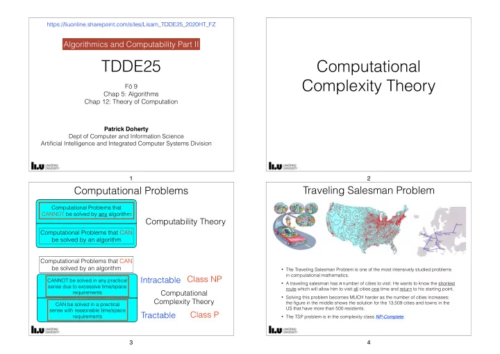
Traveling Salesman Problem
- The Traveling Salesman Problem is one of the most intensively studied problems
in computational mathematics.
- A traveling salesman has n number of cities to visit. He wants to know the shortest
route which will allow him to visit all cities one time and return to his starting point.
- Solving this problem becomes MUCH harder as the number of cities increases;
the figure in the middle shows the solution for the 13,509 cities and towns in the US that have more than 500 residents.
- The TSP problem is in the complexity class NP-Complete.
4