[PPT] - The exchange value embedded in a transport system Qinglan Xia PowerPoint Presentation

SLIDE 1

First •Prev •Next •Last •Go Back •Full Screen •Close •Quit

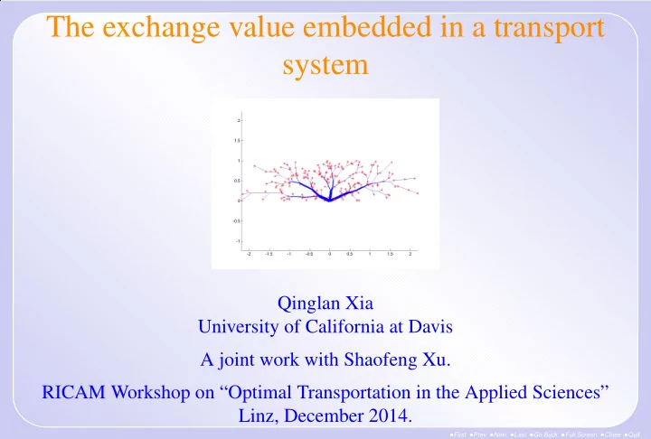
The exchange value embedded in a transport system

Qinglan Xia University of California at Davis A joint work with Shaofeng Xu. RICAM Workshop on “Optimal Transportation in the Applied Sciences” Linz, December 2014.

SLIDE 2

First •Prev •Next •Last •Go Back •Full Screen •Close •Quit

Ramified optimal transportation

Ramified optimal transportation is a closely related (but different) type of transportation to the Monge-Kantorovich problem. It aims at modeling a tree-shaped branching transport system via an optimal transport path between two probability measures. Ramified optimal transportation problem: minimize Mα(T) :=

spt(T)

θ(x)αdH1(x) among all transport path T ∈ Path(µ+, µ−), which is a rectifiable 1-current with ∂T = µ− − µ+.

SLIDE 3

First •Prev •Next •Last •Go Back •Full Screen •Close •Quit

Example: transport between atomic measures

Consider two atomic measures a =

k

i=1

miδxi and b =

ℓ

j=1

njδyj with

k

i=1

mi =

ℓ

j=1

nj = 1.

a b

V

A transport path from a to b is a polyhe- dral chain G with boundary ∂G = b − a.

SLIDE 4

First •Prev •Next •Last •Go Back •Full Screen •Close •Quit

Cost Functionals

For each G = {V (G), E(G), w : E(G) → (0, +∞)}, define the Mα mass of G by Mα (G) :=

e∈E(G)

w (e)α length (e) for some α ∈ [0, 1). Here, the length of any edge e is the Euclidean distance between its end- points.

SLIDE 5

First •Prev •Next •Last •Go Back •Full Screen •Close •Quit

SLIDE 6

First •Prev •Next •Last •Go Back •Full Screen •Close •Quit

SLIDE 7

First •Prev •Next •Last •Go Back •Full Screen •Close •Quit

SLIDE 8

First •Prev •Next •Last •Go Back •Full Screen •Close •Quit

SLIDE 9

First •Prev •Next •Last •Go Back •Full Screen •Close •Quit

SLIDE 10

First •Prev •Next •Last •Go Back •Full Screen •Close •Quit

SLIDE 11

First •Prev •Next •Last •Go Back •Full Screen •Close •Quit

SLIDE 12

First •Prev •Next •Last •Go Back •Full Screen •Close •Quit

SLIDE 13

First •Prev •Next •Last •Go Back •Full Screen •Close •Quit

SLIDE 14

First •Prev •Next •Last •Go Back •Full Screen •Close •Quit

SLIDE 15

First •Prev •Next •Last •Go Back •Full Screen •Close •Quit

SLIDE 16

First •Prev •Next •Last •Go Back •Full Screen •Close •Quit

SLIDE 17

First •Prev •Next •Last •Go Back •Full Screen •Close •Quit

SLIDE 18

First •Prev •Next •Last •Go Back •Full Screen •Close •Quit

SLIDE 19

First •Prev •Next •Last •Go Back •Full Screen •Close •Quit

SLIDE 20

First •Prev •Next •Last •Go Back •Full Screen •Close •Quit

SLIDE 21

First •Prev •Next •Last •Go Back •Full Screen •Close •Quit

SLIDE 22

First •Prev •Next •Last •Go Back •Full Screen •Close •Quit

SLIDE 23

First •Prev •Next •Last •Go Back •Full Screen •Close •Quit

Transport plan

Recall that a transport plan from a to b is an atomic probability measure q =

k

i=1

ℓ

j=1

qijδ(xi,yj) (1)

n the product space X × X such that for each i and j, qij ≥ 0,

k

i=1

qij = nj and

ℓ

j=1

qij = mi. (2) Denote Plan (a, b) as the space of all transport plans from a to b. In a transport plan q, the number qij denotes the amount of commodity re- ceived by household j from factory i.

SLIDE 24

First •Prev •Next •Last •Go Back •Full Screen •Close •Quit

A matrix associated with a transport path

Let G be a transport path in Path (a, b). We assume that for each xi and yj, there exists at most one directed polyhedral curve gij from xi to yj. In other words, there exists a list of distinct vertices V

gij
:=
vi1, vi2, · · · , vih
(3)

in V (G) with xi = vi1, yj = vih, and each

vit, vit+1
is a directed edge in

E (G) for each t = 1, 2, · · · , h − 1. This assumption clearly holds when G contains no cycles. For some pairs of (i, j), such a curve gij from xi to yj may fail to exist, due to reasons like geographical barriers, law restrictions,

etc. If such curve does not exist, we set gij = 0 to denote the empty directed

polyhedral curve. By doing so, we construct a matrix g =

gij
k×ℓ

(4) with each element of g being a polyhedral curve.

SLIDE 25

First •Prev •Next •Last •Go Back •Full Screen •Close •Quit

A simple example

A transport path from 4δx1 + 3δx2 + 4δx3 to 3δy1 + 5δy2 + 3δy3 with g13 = 0, g31 = 0. For any transport path G ∈ Path (a, b), such a matrix g =

gij
is uniquely

determined.

SLIDE 26

First •Prev •Next •Last •Go Back •Full Screen •Close •Quit

Compatibility between plan and path

Let G ∈ Path (a, b) be a transport path and q ∈ Plan (a, b) be a transport

plan. The pair (G, q) is compatible if qij = 0 whenever gij = 0 and

G = q · g. (5) Here, equation (5) means that as polyhedral chains, G =

k

i=1

ℓ

j=1

qij · gij, where the product qij ·gij denotes that an amount qij of commodity is moved along the polyhedral curve gij from factory i to household j. In terms of edges, it says that for each edge e ∈ E (G), we have

e⊆gij

qij = w (e) .

SLIDE 27

First •Prev •Next •Last •Go Back •Full Screen •Close •Quit

Compatible pair of transport path and plan

For instance, the transport path in previous example can be expressed as G = 2g11 + 2g12 + g21 + g22 + g23 + 2g32 + 2g33, (6) which means that the transport plan q = 2δ(1,1) + 2δ(1,2) + δ(2,1) + δ(2,2) + δ(2,3) + 2δ(3,2) + 2δ(3,3) is compatible with G in (6).

SLIDE 28

First •Prev •Next •Last •Go Back •Full Screen •Close •Quit

Example

Roughly speaking, the compatibility conditions check whether a transport plan is realizable by a transport path. a =1 4δx1 + 3 4δx2 and b =5 8δy1 + 3 8δy2, and consider a transport plan q = 1 8δ(x1,y1) + 1 8δ(x1,y2) + 1 2δ(x2,y1) + 1 4δ(x2,y2) ∈ Plan (a, b) . (7) It is straight forward to see that q is compatible with G1 but not G2. This is because there is no directed curve g12 from factory 1 to household 2 in G2.

SLIDE 29

First •Prev •Next •Last •Go Back •Full Screen •Close •Quit

A transport path ¯

G compatible with all plans

Example. Let x∗ ∈ X \ {x1, · · · , xk, y1, · · · , yℓ}. We may construct a path

¯ G ∈ Path (a, b) as follows. Let V ¯ G

= {x1, · · · , xk} ∪ {y1, · · · , yℓ} ∪ {x∗} ,

E ¯ G

= {[xi, x∗] : i = 1, · · · , k} ∪
x∗, yj
: j = 1, · · · , ℓ
,

and w ([xi, x∗]) = mi, w

x∗, yj
= nj

for each i and j. In this case, each gij is the union of two edges [xi, x∗] ∪

x∗, yj
. Then, each transport plan q ∈ Plan (a, b) is compatible with ¯

G.

SLIDE 30

First •Prev •Next •Last •Go Back •Full Screen •Close •Quit

Motivations

As an illustration, we consider a spacial economy with two goods located at two distinct points {x1, x2} and two consumers living at two different locations {y1, y2}.

Consumer 1 favors good 2 more than good 1. However, good 2 may be

more expensive than good 1 for some reason such as a higher transporta- tion fee.

As a result, she buys good 1 despite the fact that it is not her favorite.
On the contrary, consumer 2 favors good 1 but ends up buying good 2, as

good 1 is more expensive than good 2 for him.

SLIDE 31

First •Prev •Next •Last •Go Back •Full Screen •Close •Quit

Motivations

Given this purchase plan, a traditional trans- porter will ship the ordered items in a trans- port system like G1. However, in ramified (i.e. branching) optimal transportation, a transport system like G2 with some branching structure might be more cost efficient than G1. One may save some trans- portation cost by using a transport system like G2 instead of G1. Advantage of G2 over G1:

G2 might be more cost efficient than G1: one may save some transportation

cost by using a transport system like G2 instead of G1.

Now, we observe another very interesting advantage about G2.

SLIDE 32

First •Prev •Next •Last •Go Back •Full Screen •Close •Quit

Exchange: a happier life for free!

Unlike a traditional transport system G1, a ramified transport system G2 pro- vides an exchange value: one can simply switch the items which leads to consumer 1 getting good 2 and consumer 2 receiving good 1.

This exchange of items makes both consumers better off since they both

get what they prefer.

More importantly, no extra transportation cost is incurred during this ex-

change process. In other words, a ramified transport system like G2 may possess an exchange value, which cannot be found in a traditional transport system G1. How shall we quantify the exchange value for a ramified transport system?

SLIDE 33

First •Prev •Next •Last •Go Back •Full Screen •Close •Quit

Economy E = (U, P, W; x, y)

X: a compact convex subset of a Euclidean space Rm.
k types of goods i = 1, · · · , k located at sources {x1, · · · , xk} ⊆ X.
ℓ consumers located at y1, · · · , yℓ.
Each consumer j derives utility from consuming k goods according to a

utility function uj : Rk

+ → R :

q1j, ..., qkj
→ uj, j = 1, ..., ℓ, where

uj : Rk

+ → R is continuous, concave and increasing, j = 1, ..., ℓ.

Each consumer j has an initial wealth wj > 0 and faces a price vector

pj =

p1j, ..., pkj
∈ Rk

++, j = 1, ..., ℓ.

We allow the prices to vary across consumers to accommodate the situ-

ation where consumers on different locations may have to pay different prices for the same good. This variation could be possibly due to different transportation fees.

SLIDE 34

First •Prev •Next •Last •Go Back •Full Screen •Close •Quit

Consumer’s Problem

Each consumer j will choose an utility maximizing consumption plan given the price pj and wealth wj. More precisely, the consumption plan ¯ qj is de- rived from the following utility maximizing problem: ¯ qj ∈ arg max

uj
qj
| qj ∈ Rk

+, pj · qj ≤ wj

.

(8) Given the continuity and concavity of uj, we know this problem has a solu- tion.

SLIDE 35

First •Prev •Next •Last •Go Back •Full Screen •Close •Quit

Expenditure minimizing problem

For a given utility level ˜ uj > uj (0): ej

pj, ˜

uj

= min
pj · qj | qj ∈ Rk

+, uj

qj
≥ ˜

uj

,

(9) This is actually a problem dual to the above utility maximization problem. The continuity and concavity of uj guarantee a solution to this minimization

problem. Here, ej
pj, ˜

uj

represents the minimal expenditure needed for

consumer j to reach a utility level ˜

uj. Since ˜

uj > uj (0), we know that ej

pj, ˜

uj

> 0.

SLIDE 36

First •Prev •Next •Last •Go Back •Full Screen •Close •Quit

The least total expenditure

For each probability measure q =

qij
∈ P (X × X), we define

S (q) =

ℓ

j=1

ej

pj, uj
qj
=

ℓ

j=1

min

pj · tj | tj ∈ Rk

+, uj

tj
≥ uj
qj
,

(10) where qj =

q1j, q2j, ..., qkj
for each j = 1, · · · , ℓ. Here, S (q) represents

the least total expenditure for each individual j to reach utility level uj

qj
.
Lemma. Suppose each uj is continuous, concave, and increasing on Rk

+,

j = 1, ..., ℓ. The function S (q) is

1. Homogeneous of degree one in p = (p1, ..., pℓ) .
2. Increasing in q and nondecreasing in pij for any i = 1, ..., k, j = 1, ..., ℓ.
3. Concave in p.
4. Continuous in p and q.

SLIDE 37

First •Prev •Next •Last •Go Back •Full Screen •Close •Quit

The feasible set of G

Let ¯ q ∈ Plan (a, b) be the initial plan given by solving the utility maximiza- tion problem. Denote Ω (¯ q) = {G ∈ Path (a, b) | (G, ¯ q) is compatible} . (11) Let G ∈ Ω (¯ q) be fixed and g =

gij
be the corresponding matrix of G as

given in (4). That is, G = g · ¯ q. Then, we introduce the following definition:

Definition. Each transport plan in the set

FG =

q ∈ P (X × X)
q is compatible with G

uj

qj
≥ uj
¯

qj

, j = 1, ..., ℓ.
(12)

is called a feasible plan for G, and the set FG is called the feasible set of G.

SLIDE 38

First •Prev •Next •Last •Go Back •Full Screen •Close •Quit

The feasible set

Recall that q is compatible with G means that qij = 0 if gij does not exist (13) and g · q = g · ¯ q, in the sense that for each edge e ∈ E (G), we have an equality

e⊆gij

qij = w (e) , where w (e) =

e⊆gij

¯ qij. (14) Note that the compatibility condition ensures that replacing ¯ q by any feasible plan q ∈ FG will not change the transportation cost Mα (G), as the quantity

n each edge e of G is set to be w (e).

SLIDE 39

First •Prev •Next •Last •Go Back •Full Screen •Close •Quit

The feasible set

For any feasible plan q ∈ FG, the constraint uj

qj
≥ uj
¯

qj

means that qj

is at least as good as ¯ qj for each consumer j. Since ¯ q ∈ Plan (a, b), the compatibility condition automatically implies that q ∈ Plan (a, b) whenever q ∈ FG.

Lemma. FG is a nonempty, convex and compact subset of P (X × X) .

SLIDE 40

First •Prev •Next •Last •Go Back •Full Screen •Close •Quit

Exchange value

Definition. Let E be an economy as before. For each transport path G ∈

Ω (¯ q), we define the exchange value of G by V (G; E) = max

q∈FG

S (q) − S (¯ q) , (15) where S is given by (10). Without causing confusion, we may simply denote V (G; E) by V (G).

SLIDE 41

First •Prev •Next •Last •Go Back •Full Screen •Close •Quit
For each q ∈ FG, given uj
qj
≥ uj
¯

qj

for all j, we have

S (q) ≥ S (¯ q) . (16)

Since S is a continuous function on a compact set, the exchange value

function V : Ω (¯ q) → [0, ∞) is well defined.

Our way of defining the feasibility set FG guarantees that the exchange

value is not obtained at the expense of increasing transportation cost Mα(G).

For any G ∈ Ω (¯

q), the exchange value is always nonnegative and bounded from above: 0 ≤ V (G) ≤ V ¯ G

.

SLIDE 42

First •Prev •Next •Last •Go Back •Full Screen •Close •Quit

Exchange values in the motivational example

Let’s return to the example discussed in introduction. More precisely, sup- pose u1 (q11, q21) = q11 + 3q21, w1 = 1/2, p1 = (1, 6) and u2 (q12, q22) = 3q12 + q22, w2 = 1/2, p2 = (6, 1) . By solving (8), i.e. ¯ q1 ∈ arg max {u1 (q11, q21) | p1 · q1 ≤ w1} = arg max {q11 + 3q21 | q11 + 6q21 ≤ 1/2} = {(1/2, 0)} , we find ¯ q1 = (1/2, 0). Similarly, we have ¯ q2 = (0, 1/2). This gives the initial plan ¯ q = 1/2 1/2

.

SLIDE 43

First •Prev •Next •Last •Go Back •Full Screen •Close •Quit

Now, solving expenditure minimization problems (9) yields e1 (p1, ˜ u1) = min

p1 · q1 | q1 ∈ R2

+, u1 (q1) ≥ ˜

u1

= min
q11 + 6q21 | (q11, q21) ∈ R2

+, q11 + 3q21 ≥ ˜

u1

= ˜

u1. Similarly, we have e2 (p2, ˜ u2) = ˜

u2. From these, we get

S (q) = e1 (p1, u1 (q1)) + e2 (p2, u2 (q2)) = u1 (q1) + u2 (q2) for each probability measure q ∈ P (X × X). Now, we find the exchange value embedded in the transport systems G1 and G2.

SLIDE 44

First •Prev •Next •Last •Go Back •Full Screen •Close •Quit

Exchange value in G1 :

The associated feasible set is FG1 =   q = q11 q12 q21 q22

∈ P (X × X)
q11 = 1/2, q21 = 0, q12 = 0, q22 = 1/

q11 + 3q21 ≥ u1 (¯ q1) = 1/2, 3q12 + q22 ≥ u2 (¯ q2) = 1/2. Thus, the exchange value of G1 is V (G1) = max

q∈FG1

S (q) − S (¯ q) = S (¯ q) − S (¯ q) = 0.

SLIDE 45

First •Prev •Next •Last •Go Back •Full Screen •Close •Quit

Exchange value in G2 : The associated feasible set is

FG2 =        q = q11 q12 q21 q22

∈ P (X × X)
q11 + q12 = 1/2, q21 + q22 = 1/2,

q11 + q21 = 1/2, q11 + 3q21 ≥ u1 (¯ q1) = 1/2, 3q12 + q22 ≥ u2 (¯ q2) = 1/2.        =

q =
q11

1/2 − q11 1/2 − q11 q11

q11 ≤ 1/2

q11 ≥ 0 .

Thus, we have the following exchange value

V (G2) = max

q∈FG2

S (q) − S (¯ q) = max

q∈FG2

{(q11 + 3q21) + (3q12 + q22)} − 1 = max

0≤q11≤1

2

{(q11 + 3 (1/2 − q11)) + (3 (1/2 − q11) + q11)} − 1 = max

0≤q11≤1

2

{3 − 4q11} − 1 = 2.

SLIDE 46

First •Prev •Next •Last •Go Back •Full Screen •Close •Quit
A positive exchange value of a transport system indicates that there exists

some extra value embedded in the system by some exchange of goods between consumers.

For this consideration, we will explore explicit conditions ensuring a pos-

itive exchange value.

Basically, there are three factors affecting the exchange value: transport

structures, preferences and prices.

In the rest, we will study how these three factors affect the exchange value,

and in particular the existence of a positive exchange value.

SLIDE 47

First •Prev •Next •Last •Go Back •Full Screen •Close •Quit

Transport Structures and Exchange Value

For any G ∈ Ω (¯ q), define K (¯ q, G) = {q ∈ P (X × X) |q is compatible with G} , and U (¯ q) =

q ∈ P (X × X)
uj
qj
≥ uj
¯

qj

, j = 1, ..., ℓ.
Then,

FG = K (¯ q, G) ∩ U (¯ q) . Clearly, the structure of a transport system influences the exchange value through K (¯ q, G) . So, we focus on the properties of K (¯ q, G).

Proposition. K (¯

q, G) is a polygon of dimension N (G) + χ (G) − (k + ℓ), where χ (G) is the Euler Characteristic number of G, and N (G) is the total number of existing gij’s in G.

SLIDE 48

First •Prev •Next •Last •Go Back •Full Screen •Close •Quit
Corollary. Suppose G ∈ Ω (¯

q).

1. If k + ℓ ≥ N (G) + χ (G), then FG = {¯

q}.

2. If k+ℓ < N (G)+χ (G) and ¯

q is an interior point of the polygon K (¯ q, G), then FG is a convex set of positive dimension. In particular, FG = {¯ q} .

Proof. If k + ℓ ≥ N (G) + χ (G), the convex polygon K (¯

q, G) becomes a dimension zero set, and thus FG = {¯ q}. When k + ℓ < N (G) + χ (G), the polygon K (¯ q, G) has a positive dimension. Since each uj is concave, U (¯ q) is a convex set containing ¯

q. When ¯

q is an interior point of K (¯ q, G), the intersection FG = K (¯ q, G)∩U (¯ q) is still a convex set of positive dimension. Thus, FG = {¯ q}.

SLIDE 49

First •Prev •Next •Last •Go Back •Full Screen •Close •Quit
Proposition. Suppose G ∈ Ω (¯

q) satisfies the following condition: for any two pairs (i1, i2) with i1 = i2 and (j1, j2) with j1 = j2, we have V

gi1j2
∩ V
gi2j1
= ∅,

(17) where V

gij
is given in (3). Then, k + ℓ ≥ N (G) + χ (G). Hence, by

Corollary , FG is a singleton {¯ q}.

Proposition. If G1 is topologically equivalent to G2, then V (G1) = V (G2).

As will be clear in the next section, the topological invariance of V is a very useful result because it enables us to inherit many existing theories in ram- ified optimal transportation when studying a new optimal transport problem there.

SLIDE 50

First •Prev •Next •Last •Go Back •Full Screen •Close •Quit

Preferences and Exchange Value

Here, we study the implications of preferences, which are represented by utility functions, on the exchange value. The following proposition shows that the exchange value is zero when all consumers derive their utilities solely from the total amount of goods they consume.

Proposition. If uj : Rk

+ → R is of the form uj

qj
= fj

k

i=1 qij

for

some fj : [0, ∞) → R for each j = 1, ..., ℓ, then V (G) = 0 for any G ∈ Ω (¯ q). From this proposition, we see that a positive exchange value may fail to exist for arbitrary utility functions.

SLIDE 51

First •Prev •Next •Last •Go Back •Full Screen •Close •Quit
Proof. For any q ∈ FG, by compatibility, we know

k

i=1

qij =

k

i=1

¯ qij, j = 1, ..., ℓ, which implies uj

qj
= fj

 

k

i=1

qij   = fj  

k

i=1

¯ qij   = uj

¯

qj

,

showing that all consumers find any feasible plan indifferent to ¯

q. Therefore,

we get V (G) = max

q∈FG

S (q) − S (¯ q) = 0.

SLIDE 52

First •Prev •Next •Last •Go Back •Full Screen •Close •Quit

The solution set Q (G)

For any G ∈ Ω (¯ q), denote Q (G) as the solution set of the maximization problem (15) defining exchange value, i.e., Q (G) = {ˆ q ∈ FG | V (G) = S (ˆ q) − S (¯ q)} . (18) We are interested in describing geometric properties of the set Q (G). In particular, if Q (G) contains only one element, then the problem (15) has a unique solution.

SLIDE 53

First •Prev •Next •Last •Go Back •Full Screen •Close •Quit
Proposition. For any G ∈ Ω (¯

q) ,

1. The solution set Q (G) is a compact nonempty set.
2. If uj : Rk

+ → R is homogeneous of degree βj > 0 and

uj
qj

1

βj is

concave in qj, j = 1, ..., ℓ, then Q (G) is convex.

3. (Uniqueness) If uj : Rk

+ → R is homogeneous of degree βj > 0

and

uj
qj

1

βj is concave in qj satisfying the condition

uj
1 − λj
˜

qj + λj ˆ qj 1

βj >

1 − λj

uj

˜

qj 1

βj + λj

uj
ˆ

qj 1

βj

(19) for each λj ∈ (0, 1), and any non-collinear ˜ qj, ˆ qj ∈ Rk

+ , for each j =

1, ..., ℓ. Then Q (G) is a singleton, and thus the problem (15) has a unique solution.

SLIDE 54

First •Prev •Next •Last •Go Back •Full Screen •Close •Quit

Two classes of utility functions widely used in economics satisfy conditions in Proposition (). One is Cobb-Douglas function u : Rk

+ → R : u (q1, ..., qk) = k

i=1

(qi)τi , τi > 0, i = 1, ..., k. The other is Constant Elasticity of Substitution function u : Rk

+ → R : u (q1, ..., qk) =

 

k

i=1

γi (qi)τ  

β τ

, τ ∈ (0, 1), β > 0, γi > 0, i = 1

Proposition. Suppose uj : Rk

+ → R is homogeneous of degree βj > 0 and

uj
qj

1

βj is concave in qj satisfying (19) for each j = 1, ..., ℓ. For any

G ∈ Ω (¯ q) , V (G) > 0 if and only if FG = {¯ q}.

SLIDE 55

First •Prev •Next •Last •Go Back •Full Screen •Close •Quit
Proof. Trivially, in general, FG = {¯

q} implies V (G) = 0. On the other hand, suppose V (G) = maxq∈FG S (q) − S (¯ q) = 0, then by (16), we have S (q) = S (¯ q) for each q ∈ FG. This implies Q (G) = FG. By the uniqueness result, FG is a singleton {¯ q}. This proposition says that each transport path G ∈ Ω (¯ q) has a positive exchange value as long as FG contains more than one element. Neverthe- less, the result may fail if we drop the assumptions on the utility functions. For instance, when k > 1, ℓ > 1, let G = ¯ G as defined in Example , and uj

qj
= fj

k

i=1 qij

for some functions fj : [0, 10] → R (e.g.

fj (x) = −x2 + 20x + 100) for all j. Then, FG = Plan (a, b) = {¯ q}, but V (G) = 0 by Proposition .

SLIDE 56

First •Prev •Next •Last •Go Back •Full Screen •Close •Quit

Existence of positive exchange value

Theorem. Suppose uj : Rk

+ → R is homogeneous of degree βj > 0 and

uj
qj

1

βj is concave in qj satisfying (19) for each j = 1, ..., ℓ.

If k + ℓ < N (G) + χ (G) and ¯ q is an interior point of the polygon K (¯ q, G), then V (G) > 0.

SLIDE 57

First •Prev •Next •Last •Go Back •Full Screen •Close •Quit

Prices and Exchange Value

Here, we study the implications of prices on the exchange value. The follow- ing proposition shows that the exchange value is zero when the price vectors are collinear.

Proposition. If the price vectors are collinear, i.e., pj = λjp1, for some λj >

0, j = 1, ..., ℓ, then V (G) = 0 for any G ∈ Ω (¯ q).

Corollary. If there is only one good (k = 1) or one consumer (ℓ = 1), then

V (G) = 0 for any G ∈ Ω (¯ q).

Proof. When k = 1, define λj = pj

p1 > 0, j = 1, ..., ℓ. The result follows from

the Proposition. When ℓ = 1, for any G ∈ Ω (¯ q) , the feasible set is FG = {q1 = (q11, · · · , qk1) ∈ Plan (a, b) |qi1 = mi = ¯ qi1 for each i} = {¯ q1} , which clearly yields V (G) = 0.

SLIDE 58

First •Prev •Next •Last •Go Back •Full Screen •Close •Quit

In the following Proposition, we show that non-degeneracy conditions on the utility with respect to the transport plan which, together with some order con- ditions on prices as well as some cross-intersection conditions on polyhedral curves, ensure a positive exchange value.

Proposition. Let k = 2 and ℓ = 2. Suppose uj is differentiable at ¯

q with ∇uj

¯

qj

> 0, j = 1, 2 and ¯

qij > 0 for each i, j. If G ∈ Ω (¯ q) with V (g12) ∩ V (g21) = ∅, and p21 > p11, p12 > p22, (20) then V (G) > 0.

SLIDE 59

First •Prev •Next •Last •Go Back •Full Screen •Close •Quit

Another existence theorem on positive exchange value

Theorem. Suppose uj is differentiable at ¯

q with ∇uj

¯

qj

∈ Rk

++, j =

1, ..., ℓ, and ¯ q ∈ Rkℓ

++. If there exist some i1 = i2 ∈ {1, ..., k}, j1 = j2 ∈

{1, ..., ℓ} satisfying pi2j1 > pi1j1, pi1j2 > pi2j2 and V

gi1j2
∩ V
gi2j1
= ∅

for G ∈ Ω (¯ q), then V (G) > 0.

SLIDE 60

First •Prev •Next •Last •Go Back •Full Screen •Close •Quit

Conclusion

We’ve seen how transport structures, preferences and prices jointly deter-

mine the exchange value.

Each of these factors may lead to a zero exchange value under very rare
situations. More precisely, the exchange value is zero if

– the structure of the system yields a singleton feasible set FG, or – the utility functions are merely quantity dependent, or – price vectors are collinear across consumers.

However, under more regular situations, there exists a positive exchange

value for a ramified transport system. For instance, – if the utility functions satisfy the conditions in (3) with a non-singleton feasible set FG or – the transport systems are of ramified structures with some order condi- tions on prices and non-degeneracy conditions on the utility.

SLIDE 61

First •Prev •Next •Last •Go Back •Full Screen •Close •Quit

A New Optimal Transport Problem

Problem. Given two atomic probability measures a and b on X in a given

economy E, find a minimizer of Hα,σ (G) := Mα (G) − σV (G) (21) among all G ∈ Ω (¯ q), where Ω (¯ q) is given by (11), and α ∈ [0, 1) and σ ≥ 0 are fixed constants.

SLIDE 62

First •Prev •Next •Last •Go Back •Full Screen •Close •Quit
When the utility functions are merely quantity dependent or when price

vectors are collinear across consumers , the exchange value of any G ∈ Ω (¯ q) is always zero. In these cases, Hα,σ (G) = Mα (G) for any σ. Thus, the study of Hα,σ coincides with that of Mα.

However, it is quite possible that Hα,σ does not agree with Mα on Ω (¯

q) for σ > 0 in a general economy E.

As V is topologically invariant , many results that can be found in literature

about Mα still hold for Hα,σ. For instance, – the Melzak algorithm for finding an Mα minimizer ([?], [?], [?]) in a fixed topological class still applies to Hα,σ because V (G) is simply a constant within each topological class. – the balance equation still holds, one can still calculate angles between edges at each vertex using existing formulas, and then get a universal upper bound on the degree of vertices on an optimal Hα,σ path.

SLIDE 63

First •Prev •Next •Last •Go Back •Full Screen •Close •Quit

New situation

However, due to the existence of exchange value, one may possibly favor an

ptimal Hα,σ path instead of the usual optimal Mα path when designing a

transport system. The topological type of the optimal Hα,σ path may differ from that of the optimal Mα path. This observation is illustrated by the following example.

SLIDE 64

First •Prev •Next •Last •Go Back •Full Screen •Close •Quit

Three topologically different transport systems.

Example. Let us consider the transportation from two sources to two con-

sumers.

If we only consider minimizing Mα transportation cost, each of the three

topologically different types may occur.

However, when σ is sufficiently large, only G2 may be selected under suit-