The Integrated ARMA model: ARIMA ( p, d, q ) Some series are - - PowerPoint PPT Presentation

the integrated arma model arima p d q some series are
SMART_READER_LITE
LIVE PREVIEW

The Integrated ARMA model: ARIMA ( p, d, q ) Some series are - - PowerPoint PPT Presentation

The Integrated ARMA model: ARIMA ( p, d, q ) Some series are nonstationary, but their differences are sta- tionary; e.g. the random walk. Recall: the first differences of x t are x t x t 1 = (1 B ) x t = x t . The second


slide-1
SLIDE 1

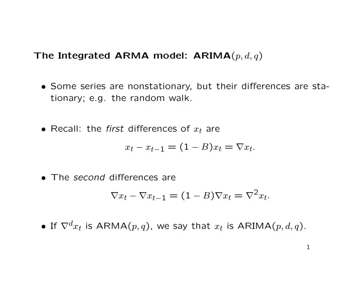
The Integrated ARMA model: ARIMA(p, d, q)

  • Some series are nonstationary, but their differences are sta-

tionary; e.g. the random walk.

  • Recall: the first differences of xt are

xt − xt−1 = (1 − B)xt = ∇xt.

  • The second differences are

∇xt − ∇xt−1 = (1 − B)∇xt = ∇2xt.

  • If ∇dxt is ARMA(p, q), we say that xt is ARIMA(p, d, q).

1

slide-2
SLIDE 2

Under-differencing

  • Suppose that xt is ARIMA(p, d, q), but we analyze yt = ∇d′xt

for some d′ < d.

  • In this case, yt satisfies

∇d−d′φ(B)yt = φ∗(B)yt = θ(B)wt where φ∗(z) = (1 − z)(d−d′)φ(z) has d − d′ roots at z = 1.

  • This looks like an ARMA(p + d − d′, q) model, but it is not

causal.

2

slide-3
SLIDE 3

Over-differencing

  • Suppose that xt is ARIMA(p, d, q), but we analyze yt = ∇d′xt

for some d′ > d.

  • In this case, yt satisfies

φ(B)yt = ∇d′−dθ(B)wt = θ∗(B)wt where θ∗(z) = (1 − z)(d′−d)θ(z) has d′ − d roots at z = 1.

  • This looks like an ARMA(p, q + d′ − d) model, but it is not

invertible.

3

slide-4
SLIDE 4

Simplest model with d > 0: ARIMA(0, 1, 1)

  • Many nonstationary series are found to be fitted quite well

as ARIMA(0, 1, 1).

  • This model is connected with the exponentially weighted

moving average (EWMA) method of forecasting.

  • If the model is written xt − xt−1 = wt − λwt−1, the one-step

forecast is ˜ xn+1 = (1 − λ)

  • j=0

λjxn−j, the exponentially weighted moving average.

4

slide-5
SLIDE 5
  • We can calculate the forecast recursively:

xn+1 = xn − λwn + wn+1.

  • We can find wn from xn, xn−1, . . . , so the one-step forecast

is the first part: ˜ xn+1 = xn − λwn

5

slide-6
SLIDE 6
  • But wn is the previous forecast error, xn − ˜

xn, so ˜ xn+1 = xn − λ(xn − ˜ xn) = (1 − λ)xn + λ˜ xn.

  • In words,

the new forecast is a weighted average of the current forecast and the current value.

  • Also

˜ xn+1 = ˜ xn + (1 − λ)(xn − ˜ xn), so the new forecast is the current forecast plus a correction based on the current forecast error.

6

slide-7
SLIDE 7

Strategy for Building ARIMA Models

  • 1. First choose d:
  • ACF of an integrated series tends to die away slowly, so

difference until it dies away quickly;

  • the IACF of a non-invertible series tends to die away

slowly, which indicates over-differencing.

  • You may want to try more than one value of d.
  • 2. Next choose p and q, e.g. using MINIC.

7

slide-8
SLIDE 8
  • 3. Next estimate the model.
  • 4. Finally check the model diagnostics:
  • Significance of highest order coefficients, ˆ

φp (if p > 0) and ˆ θq (if q > 0);

  • Non-significance in autocorrelation check of residuals;
  • Low value of AIC or SBC.
  • 5. Repeat from step 2 until satisfactory.
  • Note: You may not find a completely satisfactory model,

especially for a long data series.

8

slide-9
SLIDE 9

Unit Root Tests

  • Choice of d can be formulated as a hypothesis test.
  • E.g. in the AR(1) model xt = φxt−1 + wt, set:

– H0 : φ = 1, xt is ARIMA(0, 1, 0) (nonstationary, d = 1); – HA : |φ| < 1, xt is ARIMA(1, 0, 0) (stationary, d = 0). Test using proc arima’s stationarity keyword on the identify statement.

  • E.g. the global temperature data: proc arima program and
  • utput.

9

slide-10
SLIDE 10
  • The statistics on the “Lags 0” rows in the panel “Augmented

Dickey-Fuller Unit Root Tests” refer to the three models – Zero Mean: xt = φxt−1 + wt; – Single Mean: xt − µ = φ(xt−1 − µ) + wt; – Trend: xt − µ − βt = φ

xt−1 − µ − β(t − 1) + wt.

10

slide-11
SLIDE 11
  • Note that under H0, these models reduce to

xt = xt−1 + wt, xt = xt−1 + wt, xt = xt−1 + β + wt, the first two being random walks with no drift, the latter being a random walk with drift.

  • The statistics on the “Lags 1” rows refer to corresponding

AR(2) models, which reduce to integrated AR(1) models under the null hypothesis.

  • The “Tau” tests are generally preferred to the “Rho” tests.

11

slide-12
SLIDE 12
  • E.g. Case-Shiller housing data: proc arima program and out-

put.

12