[PDF] - The middle program $ middle 3 3 5 middle: 3 $ middle 2 1 3 PDF Document

SLIDE 1

Andreas Zeller

Detecting Anomalies

2

Tracing Infections

✘

For every infection, we must find the earlier

infection that causes it.

Which origin should we focus upon?

3

Tracing Infections

✘

1 2 3

SLIDE 2

4

Focusing on Anomalies

✘

Examine origins and locations where

something abnormal happens

What’s normal?

General idea: Use induction – reasoning

from the particular to the general

Start with a multitude of runs
Determine properties that are common

across all runs

5

What’s abnormal?

Suppose we determine common properties
f all passing runs.
Now we examine a run which fails the test.
Any difference in properties correlates with

failure – and is likely to hint at failure causes

6

4 5 6

SLIDE 3

Detecting Anomalies

7

Run Run Run Run Run Run

✔ ✘

Properties Properties Differences correlate with failure

Properties

8

Data properties that hold in all runs:

“At f(), x is odd”
“0 ≤ x ≤ 10 during the run”

Code properties that hold in all runs:

“f() is always executed”
“After open(), we eventually have close()”

Comparing Coverage

1. Every failure is caused by an infection,

which in turn is caused by a defect

2. The defect must be executed to start the

infection

3. Code that is executed in failing runs only is

thus likely to cause the defect

9

7 8 9

SLIDE 4

10

The middle program

middle 3 3 5 $ middle: 3 middle 2 1 3 $ middle: 1

11

int main(int arc, char *argv[]) { int x = atoi(argv[1]); int y = atoi(argv[2]); int z = atoi(argv[3]); int m = middle(x, y, z); printf("middle: %d\n", m); return 0; }

12

int middle(int x, int y, int z) { int m = z; if (y < z) { if (x < y) m = y; else if (x < z) m = y; } else { if (x > y) m = y; else if (x > z) m = x; } return m; } 10 11 12

SLIDE 5

13

Obtaining Coverage

for C programs x 3 1 3 5 5 2 y 3 2 2 5 3 1 z 5 3 1 5 4 3

✔

✔ ✔ ✔ ✔

✘

14

int middle(int x, int y, int z) { int m = z; if (y < z) { if (x < y) m = y; else if (x < z) m = y; } else { if (x > y) m = y; else if (x > z) m = x; } return m; }

15

Discrete Coloring

executed only in failing runs executed in passing and failing runs executed only in passing runs highly suspect ambiguous likely correct

13 14 15

SLIDE 6

x 3 1 3 5 5 2 y 3 2 2 5 3 1 z 5 3 1 5 4 3

✔

✔ ✔ ✔ ✔

✘

16

int middle(int x, int y, int z) { int m = z; if (y < z) { if (x < y) m = y; else if (x < z) m = y; } else { if (x > y) m = y; else if (x > z) m = x; } return m; } x 3 1 3 5 5 2 y 3 2 2 5 3 1 z 5 3 1 5 4 3

✔

✔ ✔ ✔ ✔

✘

int middle(int x, int y, int z) { int m = z; if (y < z) { if (x < y) m = y; else if (x < z) m = y; } else { if (x > y) m = y; else if (x > z) m = x; } return m; }

17 18

Continuous Coloring

executed only in failing runs passing and failing runs executed only in passing runs

16 17 18

SLIDE 7

19

Hue

hue(s) = red hue + %passed(s) %passed(s) + %failed(s) × hue range

0% passed 100% passed

20

Brightness

frequently executed rarely executed

bright(s) = max

%passed(s), %failed(s)
x

3 1 3 5 5 2 y 3 2 2 5 3 1 z 5 3 1 5 4 3

✔

✔ ✔ ✔ ✔

✘

int middle(int x, int y, int z) { int m = z; if (y < z) { if (x < y) m = y; else if (x < z) m = y; } else { if (x > y) m = y; else if (x > z) m = x; } return m; }

21

Source: Jones et al., ICSE 2002

19 20 21

SLIDE 8

22

Source: Jones et al., ICSE 2002

23

Evaluation

How well does comparing coverage detect anomalies?

How green are the defects? (false negatives)
How red are non-defects? (false positives)

Space

8000 lines of executable code
1000 test suites with156–4700 test cases
20 defective versions with one defect each

(corrected in subsequent version)

24

22 23 24

SLIDE 9

25

18 of 20 defects are correctly classified in the “reddest” portion of the code

Source: Jones et al., ICSE 2002

26

The “reddest” portion is at most 20% of the code

Source: Jones et al., ICSE 2002

Siemens Suite

7 C programs, 170–560 lines
132 variations with one defect each
108 all yellow (i.e., useless)
1 with one red statement (at the defect)

27

Source: Renieris and Reiss, ASE 2003

25 26 27

SLIDE 10

Nearest Neighbor

28

Run Run Run Run Run Run

✔ ✘

Nearest Neighbor

29

Run Run Run Run Run Run

✔ ✘

Compare with the single run that has the most similar coverage

✔

30

Locating Defects

25 50 75 100 <10 <20 <30 <40 <50 <60 <70 <80 <90 <100 Nearest Neighbor Intersection

% of failing tests % of executed source code to examine

Renieris+Reiss (ASE 2003) Results obtained from Siemens test suite; can not be generalized Jones et al. (ICSE 2002)

28 29 30

SLIDE 11

Sequences

31

pen() read() close()

✔

pen() close() read()

✘ close() open() read() ✘

Sequences of locations can correlate with failures: …but all locations are executed in both runs!

32

The AspectJ Compiler

ajc Test3.aj $ java test.Test3 $ test.Test3@b8df17.x Unexpected Signal : 11

ccurred at PC=0xFA415A00

Function name=(N/A) Library=(N/A) ... Please report this error at http:// java.sun.com/... $

Coverage Difgerences

33

Compare the failing run with passing runs
BcelShadow.getThisJoinPointVar() is

invoked in the failing run only

Unfortunately, this method is correct

31 32 33

SLIDE 12

Sequence Difgerences

34

This sequence occurs only in the failing run:

ThisJoinPointVisitor.isRef(),

ThisJoinPointVisitor.canTreatAsStatic(), MethodDeclaration.traverse(), ThisJoinPointVisitor.isRef(), ThisJoinPointVisitor.isRef()

Defect location

Collecting Sequences

35 mark read read skip read read skip read mark read read read read skip skip read read read read skip skip read mark read read read read skip skip read

Trace Sequences Sequence Set

anInputStreamObj InputStream

Ingoing vs. Outgoing

36

aProducer aQueue aLinkedList

add add

aConsumer

isEmpty size get firstElement removeFirst isEmpty size add add add add

incoming calls

utgoing

calls aLogger

add

34 35 36

SLIDE 13

Anomalies

37

1.0 0.5 0.5 0.5 0.5 1.0 passing run passing run failing run 0.60 0.50 0.40 ranking by average weight weights

NanoXML

38

Simple XML parser written in Java
5 revisions, each with 16–23 classes
33 errors discovered or seeded

Locating Defects

39

25 50 75 100 1 2 3 4 5 6 7 8 9 AMPLE/window size 8

classes to examine (of 16) % of failing tests

n average 0.5 classes

less than window size 1

Results obtained from NanoXML; can not be generalized Dallmeier et al. (ECOOP 2005)

37 38 39

SLIDE 14

40

Properties

41

Data properties that hold in all runs:

“At f(), x is odd”
“0 ≤ x ≤ 10 during the run”

Code properties that hold in all runs:

“f() is always executed”
“After open(), we eventually have close()”

Techniques

42

Dynamic Invariants Value Ranges Sampled Values

40 41 42

SLIDE 15

Techniques

43

Dynamic Invariants Value Ranges Sampled Values

Dynamic Invariants

44

Run Run Run Run Run Run

✔ ✘

At f(), x is odd At f(), x = 2 Invariant Property

Daikon

45

Determines invariants from program runs
Written by Michael Ernst et al. (1998–)
C++, Java, Lisp, and other languages
analyzed up to 13,000 lines of code

43 44 45

SLIDE 16

public int ex1511(int[] b, int n) { int s = 0; int i = 0; while (i != n) { s = s + b[i]; i = i + 1; } return s; }

Postcondition

b[] = orig(b[]) return == sum(b)

Precondition

n == size(b[]) b != null n <= 13 n >= 7

Daikon

46

Run with 100 randomly generated arrays
f length 7–13

Daikon

47

Run Run Run Run Run Trace Invariant Invariant Invariant Invariant

✔

get trace filter invariants report results

Postcondition

b[] = orig(b[]) return == sum(b)

Getting the Trace

48

Run Run Run Run Run Trace

✔

Records all variable values at all function

entries and exits

Uses

VALGRIND to create the trace

46 47 48

SLIDE 17

Filtering Invariants

49

Trace Invariant Invariant Invariant Invariant

Daikon has a library of

invariant patterns over variables and constants

Only matching patterns are

preserved

Method Specifications

50

x = 6 x ∈ {2, 5, –30} x < y y = 5x + 10 z = 4x +12y +3 z = fn(x, y) A subseq B x ∈ A sorted(A)

using primitive data using composite data checked at method entry + exit

Object Invariants

51

string.content[string.length] = ‘\0’ node.left.value ≤ node.right.value this.next.last = this

checked at entry + exit of public methods

49 50 51

SLIDE 18

Matching Invariants

52

A == B s size(b[]) n

public int ex1511(int[] b, int n) { int s = 0; int i = 0; while (i != n) { s = s + b[i]; i = i + 1; } return s; }

sum(b[]) return

rig(n)

Pattern Variables …

== s n size (b[]) sum (b[])

rig

(n) ret s n size(b[]) sum(b[])

rig(n)

ret

Matching Invariants

53

s i n A == B s size(b[]) n sum(b[]) return

rig(n)

Pattern Variables …

run 1

✘ ✘ ✘ ✘ ✘ ✘ ✘ ✘ ✘ ✘

== s n size (b[]) sum (b[])

rig

(n) ret s n size(b[]) sum(b[])

rig(n)

ret

Matching Invariants

54

s i n A == B s size(b[]) n sum(b[]) return

rig(n)

Pattern Variables … ✘ ✘ ✘ ✘ ✘ ✘ ✘ ✘ ✘ ✘

run 2

✘ ✘ ✘ ✘ ✘ ✘ ✘ ✘ ✘ ✘

52 53 54

SLIDE 19

== s n size (b[]) sum (b[])

rig

(n) ret s n size(b[]) sum(b[])

rig(n)

ret

Matching Invariants

55

s i n A == B s size(b[]) n sum(b[]) return

rig(n)

Pattern Variables … ✘ ✘ ✘ ✘ ✘ ✘ ✘ ✘ ✘ ✘

run 3

✘ ✘ ✘ ✘ ✘ ✘ ✘ ✘ ✘ ✘

== s n size (b[]) sum (b[])

rig

(n) ret s n size(b[]) sum(b[])

rig(n)

ret

Matching Invariants

56

s == sum(b[]) ✘ ✘ ✘ ✘ ✘ ✘ ✘ ✘ ✘ ✘ ✘ ✘ ✘ ✘ ✘ ✘ ✘ ✘ ✘ ✘ s == ret n == size(b[]) ret == sum(b[])

Matching Invariants

57

s == sum(b[]) s == ret n == size(b[]) ret == sum(b[])

public int ex1511(int[] b, int n) { int s = 0; int i = 0; while (i != n) { s = s + b[i]; i = i + 1; } return s; }

55 56 57

SLIDE 20

Enhancing Relevance

Handle polymorphic variables
Check for derived values
Eliminate redundant invariants
Set statistical threshold for relevance
Verify correctness with static analysis

58

Daikon Discussed

As long as some property can be observed,

it can be added as a pattern

Pattern vocabulary determines the

invariants that can be found (“sum()”, etc.)

Checking all patterns (and combinations!)

is expensive

Trivial invariants must be eliminated

59

Techniques

60

Dynamic Invariants Value Ranges Sampled Values polymorphic variables: treat “object x” like “int x” if possible derived values: have “size (…)” as extra value to compare against redundant invariants: like x > 0 => x >= 0 statistical threshold: to eliminate random

ccurrences

verify correctness: to make sure invariants always hold

58 59 60

SLIDE 21

Dynamic Invariants

61

Run Run Run Run Run Run

✔ ✘

At f(), x is odd At f(), x = 2 Invariant Property Can we check this

n the fly?

Diduce

62

Determines invariants and violations
Written by Sudheendra Hangal and Monica

Lam (2001)

Java bytecode
analyzed > 30,000 lines of code

Diduce

63

Run Run Run Run Run Run

✔ ✘

Invariant Property Training mode Checking mode

61 62 63

SLIDE 22

Training Mode

64

Run Run Run Run Run

✔

Invariant

Start with empty set
f invariants
Adjust invariants

according to values found during run

Invariants in Diduce

For each variable, Diduce has a pair (V, M)

V = initial value of variable
M = range of values: i-th bit of M is cleared

if value change in i-th bit was observed

With each assignment of a new value W,

M is updated to M := M ∧ ¬ (W ⊗ V)

Differences are stored in same format

65

Training Example

66

Code i Values alues Differences erences Invariant

i = 10

1010 1010 1111 – – i = 10

i += 1

1011 1010 1110 1 1111 10 ≤ i ≤ 11 ∧ |i′ – i| = 1

i += 1

1100 1010 1000 1 1111 8 ≤ i ≤ 15 ∧ |i′ – i| = 1

i += 1

1101 1010 1000 1 1111 8 ≤ i ≤ 15 ∧ |i′ – i| = 1

i += 2

1111 1010 1000 1 1101 8 ≤ i ≤ 15 ∧ |i′ – i| ≤ 2

V M V M

During checking, clearing an M-bit is an anomaly

64 65 66

SLIDE 23

67

Less space and time requirements
Invariants are computed on the fly
Smaller set of invariants
Less precise invariants

Diduce vs. Daikon Techniques

68

Dynamic Invariants Value Ranges Sampled Values

Detecting Anomalies

69

Run Run Run Run Run Run

✔ ✘

Properties Properties Differences correlate with failure How do we collect data in the field?

67 68 69

SLIDE 24

Liblit’s Sampling

70

We want properties of runs in the field
Collecting all this data is too expensive
Would a sample suffice?
Sampling experiment by Liblit et al. (2003)

Return Values

Hypothesis: function return values correlate

with failure or success

Classified into positive / zero / negative

71

CCRYPT fails

CCRYPT is an interactive encryption tool
When CCRYPT asks user for information

before overwriting a file, and user responds with EOF, CCRYPT crashes

3,000 random runs
Of 1,170 predicates, only file_exists() > 0

and xreadline() == 0 correlate with failure

72

70 71 72

SLIDE 25

Liblit’s Sampling

73

Run Run Run Run Run

✔

Properties

Can we apply this

technique to remote runs, too?

1 out of 1000 return

values was sampled

Performance loss <4%

500 1000 1500 2000 2500 3000 20 40 60 80 100 120 140

Number of successful trials used Number of "good" features left

Failure Correlation

74

After 3,000 runs,

nly five predicates are left

that correlate with failure

Web Services

75

Sampling is first choice for web services
Have 1 out of 100 users run an

instrumented version of the web service

Correlate instrumentation data with failure
After sufficient number of runs, we can

automatically identify the anomaly

73 74 75

SLIDE 26

Techniques

76

Dynamic Invariants Value Ranges Sampled Values

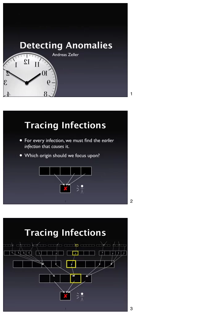
Anomalies and Causes

77

An anomaly is not a cause, but a correlation
Although correlation ≠ causation,

anomalies can be excellent hints

Future belongs to those who exploit
Correlations in multiple runs
Causation in experiments

20 40 60 80 0% <10% <20% <30%

10,0 57,0 77,0 79,0 10,0 42,0 64,0 70,0 5,0 35,0 41,0 48,0 16,0 25,0 37,0

78

Locating Defects

% of failing tests source code to examine

Results obtained from Siemens test suite; can not be generalized

NN (Renieris + Reiss, ASE 2003) CT (Cleve + Zeller, ICSE 2005) SD (Liblit et al., PLDI 2005) SOBER (Liu et al, ESEC 2005)

2 runs 5,542 runs

76 77

NN (Nearest Neighbor) @Brown by Manos Renieris + Stephen Reiss CT (Cause Transitions) @Saarland by Holger Cleve + Andreas Zeller SD (Statistical Debugging) @Berkeley by Ben Liblit (now Wisconsin), Mayur Naik (Stanford), Alice Zheng, Alex Aiken (now Stanford), Michael Jordan SOBER @Urbana- Champaign + Purdue by Liu, Yan, Fei, Han, Midkifg

78

SLIDE 27

79

Concepts

Comparing coverage (or other features) shows anomalies correlated with failure Nearest neighbor or sequences locate errors more precisely than just coverage Low overhead + simple to realize

80

Concepts (2)

Comparing data abstractions shows anomalies correlated with failure Variety of abstractions and implementations Anomalies can be excellent hints Future: Integration of anomalies + causes

81 This work is licensed under the Creative Commons Attribution License. To view a copy of this license, visit http://creativecommons.org/licenses/by/1.0

r send a letter to Creative Commons, 559 Abbott Way, Stanford, California 94305, USA.