The planned Nab/abBA/PANDA spectrometer Stefan Bae ler The - - PowerPoint PPT Presentation

the planned nab abba panda spectrometer stefan bae ler
SMART_READER_LITE
LIVE PREVIEW

The planned Nab/abBA/PANDA spectrometer Stefan Bae ler The - - PowerPoint PPT Presentation

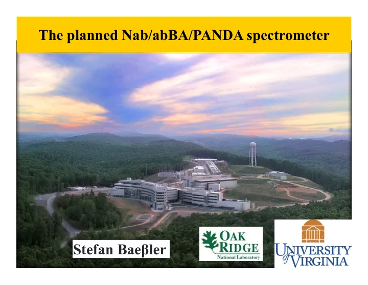
The planned Nab/abBA/PANDA spectrometer Stefan Bae ler The Spallation Neutron Source SNS in Oak Ridge, TN Linear H - accelerator Accumulator ring (buncher) Target Target Guide Hall Usage of neutrons @ SNS 7 - Engineering 11A - Powder 9


slide-1
SLIDE 1

The planned Nab/abBA/PANDA spectrometer Stefan Baeβler

slide-2
SLIDE 2

The Spallation Neutron Source SNS in Oak Ridge, TN

Linear H- accelerator Accumulator ring (buncher) Target Target Guide Hall

slide-3
SLIDE 3

Usage of neutrons @ SNS

11A - Powder Diffractometer Commission 2007 7 - Engineering Diffractometer IDT CFI Funded C i i 2008 9 – VISION 12 - Single Crystal Diffractometer Commission 2009 Commission 2008 6 - SANS Commission 2007 4B - Liquids 5 - Cold Neutron Chopper Spectrometer Commission 2007 13 - Fundamental Physics Beamline Commission 2008 4A - Magnetism Reflectometer C i i 2006 Reflectometer Commission 2006 14B - Hybrid Spectrometer Commission 2011 3 - High Pressure Diffractometer Commission 2008 Commission 2006 18 - Wide Angle 17 - High Resolution Chopper Spectrometer 15 – Spin Echo 1B - Disordered Mat’ls Commission 2010 2 - Backscattering Spectrometer Commission 2006 18 Wide Angle Chopper Spectrometer Commission 2007 Commission 2008

slide-4
SLIDE 4

Performance of FNPB beamline

Wrap-around neutrons Measured (@1 MW) neutron capture flux at FNPB beam exit:

9 c 2

1 4 10 @ 1.4 MW cm s F = ´ ⋅

slide-5
SLIDE 5

Neutron beta decay

  p+ e-

n

 n

e

slide-6
SLIDE 6

Beta Decay in the Standard Model

60Co

I  I 

e-

Fermi’s golden rule:

2 weak

2 decay probability

i f

f H i   

 

Parity Violation found by Wu et al, 1956

5

G V

e-

60Co

ud 5 F weak 5

h.c. 2 1

μ μ e

G H p γ γ γ n e γ γ γ ν V

 

    

3 Helicity 1 Quark mixing 2 Nucleon structure 3. Helicity

… of elementary fermions: –p/E,

μ

  • νμ
  • 1. Quark mixing

2

95% V

2. Nucleon structure effects

gV = GF·Vud·1 … of elementary anti- fermions: +p/E

e

 

d u s c

2 ud

95% V 

gA= GF·Vud·λ

No nuclear structure effects e-

e e

p 

b t c

(for neutrons)

slide-7
SLIDE 7

Observables in Neutron Beta Decay

p e-

n

 

e

 

Jackson et al., PR 106, 517 (1957): Observables in Neutron beta decay, as a function of generally possible coupling constants (assuming only

  

2 2 2

2 1 3 V dw G E    

p n

e

generally possible coupling constants (assuming only Lorentz-Invariance)

  

2 e e

1 3 1 b m d E p p  

   

  

d e u e

1 3

F V

G E dE     

  

2 e e e e e e e

1 3 1 + a b A B dw E E p p E E p p p p D     

   

                 

Fierz interference term b 

e e n e e

+ A B p p p p E E E E D

   

           

2

R    Beta-Asymmetry Neutrino-Electron-Correlation

2

Re 2 1 3 A       

2 2

1 a    

 

 

u 1 2 2 e 2 n d

2 1 3

F

G V E

     

Neutron lifetime

2

1 3  

slide-8
SLIDE 8

The Standard Model Parameters Vud and λ

νe

       2 1

p

Fermi-Decay: gV = GF·Vud

νe e- e-

A = 0

S = 0, mS = 0

n

Gamow-Teller-Decay:

p

       2 1

νe νe e- e-

A = 0

S = 1, mS = 0

y gA = GF·Vud·λ

p e- νe

A = -1

S = 1, mS = 1

 

n

1 cos ,

e e e

p dw A p E         

,

S (after D. Dubbers, Prog. Part. Nucl. Phys. 26, 173 (1991)

Two unknown parameters, gA and gV, need to be determined in 2 experiments

  • 1. Neutron-Lifetime:

 

1 2 2 n V A

3 g g

  

n

885 s  

2 2

2 0.1 1 3 A           

A V

g g

  • 2. Beta-Asymmetry:
slide-9
SLIDE 9

Neutron Lifetime Measurements

Decrease of Neutron Counts N with storage time t: N(t) = N(0)exp{-t/τeff} 1/ τeff = 1/τβ+1/τwall losses

895 Spivak 88 Nesvizh.92 Byrne 96 Arzumanov Nico 05 PDG2010 890 me [s] Mampe 89 00 PDG2010 Pichlmaier 10 Serebrov 08 885 Neutron lifetim Mampe 93 Serebrov 05 Serebrov 10 875 880

Many new attempts mostly with UCN in magnetic bottles: Ezhov et al (ILL PNPI Gatchina)

1988 1992 1996 2000 2004 2008 2012 Experiment publication

Many new attempts, mostly with UCN in magnetic bottles: Ezhov et al. (ILL, PNPI Gatchina), Arzumanov et al. (Kurchatov Inst., ILL), Liu et al. (Indiana), Paul et al. (TUM), Huffman et al. (NIST, NCSU), Nico et al. (NIST), Zimmer et al., (ILL) are (at least) under construction.

slide-10
SLIDE 10

The Beta Asymmetry

p+ n e-

  • 1.255

e

Electron Detector (Plastic Scintillator)

Yerozolimski Liaud PDG2010 1 265

  • 1.26

( ) Decay Electrons

PERKEO I Mostovoi PDG2010

  • 1.27
  • 1.265

λ

Polarized Neutrons Decay Electrons

PERKEO II UCNA PERKEO II, prelim

  • 1.28
  • 1.275

1985 1990 1995 2000 2005 2010 Publication year

Ongoing funded experiments:

Split Pair Magnet Magnetic Field

PERKEO II Ongoing funded experiments: UCNA (NCSU, LANL), PERKEO III (Heidelberg), PERC (Europe)

slide-11
SLIDE 11

Use of coupling constants in Primordial Nucleosynthesis

W± e- p W± νe p

Before Phase Transition: Equilibrium

W± e- p νe n

n + νe ↔ p + e-

e+ n

n + e+ ↔ p + νe

After Phase Transition (some minutes

n ↔ p + e-+ νe

νe n

After Phase Transition (some minutes after Big Bang):

n + p → d + γ d + d → 3He + n → t + p d + 3He → 4He + p d + He → He + p

Then the Primordial Nucleosynthesis stops, as there are no stable nuclei with A = 5, 8, and as h f di ….. the free neutrons die out. Stronger coupling constants in n ↔ p reactions ⇒ Phase transition later ⇒ nucleon density lower after phase transition ⇒ less 4He, more d

slide-12
SLIDE 12

Search for Standard Model Parameters

0.980 0.975

ft(0+→0+) [Hardy09] ft(0+→0+) [Liang09 – DD-ME2] Kaons +Unitarity [PDG 2010]

0.970

Vud

ft(0+→0+) [Liang09 – PKO1] PIBETA [Pocanic04]

0.965

PDG 2010] 010]

0 960

λ [P A [UCNA 20

  • 1.290
  • 1.280
  • 1.270
  • 1.260

λ = gA/gV

0.960

A [PERKEO II, prel.]

slide-13
SLIDE 13

Unitarity and superallowed nuclear decays

V Telegdi 1977:

  • V. Telegdi, 1977:

I would like to say that the theory of β-decay is the theory of the decay of the neutron. I have always thought that nuclear β-decay experiments were only done faute de mieux: … If you do not know how to do the one experiment, you take the average of twenty.

( )

2 2 2 V F ud 2 ud 2

1 2 1

V

Ft g G V V G Ft µ = µ +D

( )

F

2 1

R

G Ft +D

2 2 2

1 V V V

u ud s ub

1 V V V = -

  • (Dubbers

average)

Liang et al., PRC 79, 064316 (2009) Dubbers, Schmidt, RMP (2011), in press

slide-14
SLIDE 14

Possible Tests of the Standard Model

1 S h f Ri ht h d d C t (l t i hth d d) W ? Multiple determinations (nuclear physics, other correlation coefficients)

  • verconstrain problem, enable:
  • 1. Search for Right-handed Currents (leptons are righthanded): WR?
  • 2. Search for Scalar and Tensor interactions (neutrinos have opposite

handedness to electrons – 4 new coupling constants possible): Leptoquarks? Charged Higgs Bosons? Supersymmetry?

  • 3. Test of the Unitarity of the Cabbibo-Kobayashi-Maskawa-Matrix:

ud u ub s

d' d V V V            

Extra Z bosons? Supersymmetry? 4th quark generation?

2

95% V cd cs cb td td tb

s' s b' b V V V V V V                          

d u s c

2 ud

95% V 

2 us

5% V  us 2 2 ub u 2 d

1 ? V V V + + = +

b t c

2 ub

0.000015 V 

slide-15
SLIDE 15

Determination of the Coupling Constants

νe

       2 1

p

Fermi-Decay: gV = GF·Vud

νe e- e-

a = 1

n

Gamow-Teller-Decay:

p

       2 1

νe νe e- e-

a = 1

y gA = GF·Vud·λ

p e- νe

a = -1

 

1 cos ,

e

e

v dw a p p c

       

Two unknown parameters, gA and gV, need to be determined in 2 experiments

  • 1. Neutron-Lifetime:

 

1 2 2 n V A

3 g g

  

n

885 s    

A V

g g

  • 2b. Neutrino-Electron-Correlation a:

2 2

1 ~ 0.1 1 3       a

slide-16
SLIDE 16

e-

Idea of the cos θeν spectrometer Nab @ SNS

p  

n e

e 

 p Kinematics:

  • Energy Conservation:
  • Momentum Conservation

e,max e

E E E

 

 Proton phase space (Dalitz plot) Probability (arb. units) 1 5

1 cos

e e e

p dw a E

        

e

  • Momentum Conservation

2 2 2 e e p

2 cos

e

p p p p p

  

    cos θeν = 1 Proton phase space (Dalitz plot) Probability (arb. units) 1 1.25 1.5 Ee = 236 keV 700 keV [MeV2/c2] 0.75 1 75 keV  

 

2 2 p e min, max

Edges: Slope: p p p

 

pp

2 [

0.25 0.5 cos θeν = 0 cos θeν = -1 450 keV  

2 e p e

Slope: 1 cos

e

p a p E

        

Ee [MeV] 0.2 0.4 0.6 0.8 Alternative approaches: aSPECT (Mainz, ILL), aCORN (Tulane, NIST)

slide-17
SLIDE 17

The asymmetric version of Nab @ SNS

30 kV

Advantages of asymmetric configuration: D i f i I d fli h h

Segmented Si detector TOF region

  • Detection function: Improved flight path

length

  • Reduced sensitivity to electrostatic and

ti t ti l i h iti

magnetic filter region (field B0) g (field rB·B0)

magnetic potential inhomogeneities

  • Avoid deep Penning trap
  • Statistical uncertainty: Bigger decay

decay volume (field rB,DV·B0) 0 kV

y gg y volume vs. angular acceptance

  • Polarized experiment (abBA, PANDA)

still possible

0 kV 0 kV Neutron beam 0 kV

slide-18
SLIDE 18

The cosθeν spectrometer Nab @ SNS

ution

 

2 e p e

1 cos

e

p a p E

 

Segmented Si detector

  • 30 kV

pp

2 distribu

 

2 p

cos 1

e

p

  

 

2 p

cos 1

e

p

  

magnetic filter i (fi ld B ) TOF region (field rB·B0)

107

pp

2 [MeV2/c2]

0.0 0.5 1.0 1.5

Ee = 550 keV

region (field B0) decay volume (field rB,DV·B0)

nt rate

106 107

Neutron beam 0 kV

Simulated coun Ee = 300 keV

104 105

Ee = 500 keV

  • Measurement of Ee and tp for each event

B k d i th h i id f l t d

0 kV

0.00 0.02 0.04 0.06 0.08

1/tp

2 [1/μs2]

103 10

Ee = 700 keV

  • Background suppression through coincidences of electron and

proton.

  • Long flight path improves spectrometer
slide-19
SLIDE 19

Determination of pp through tp: The magnetic field

30 kV

p

||

p

z Segmented Si detector TOF region Magnetic Field

abatic ersion

x magnetic filter region (field B0) g (field rB·B0) Proton Trajectory

Adia conv

z decay volume (field rB,DV·B0) 0 kV

p

||

p

x 0 kV 0 kV Neutron beam z

  • Measurement of Ee and tp for each

event

  • Background suppression through

0 kV x

g pp g coincidences of electron and proton.

  • Long flight path improves

spectrometer

slide-20
SLIDE 20

Silicon detector for Nab / abBA / PANDA

Front side Back side

Segmented ion-implanted silicon detector with fast readout electronics:

  • Thickness 2 mm (less for testing)
  • Thin dead layer of < 100 nm silicon (measured!):
  • Thin dead layer of < 100 nm silicon (measured!):

Energy loss for 30 keV protons: < 11 keV (measured!)

  • 127 channels

Sufficiently small count rate/pixel, Allows to find electron and correlated proton.

slide-21
SLIDE 21

Detector properties: proton response

Proton beam, 32 keV, 50 s-1 Detector thickness: 500 μm

slide-22
SLIDE 22

Detector properties: proton spectrum (II)

ld

10

3

10

4

10

5

average energy loss: 11 keV

Threshold?

Worst case simulation (dead layer: 100 nm Si)

Energy calibration: Si 1.0mm detector Yiel

10

1

10

2

10

3

Energy calibration: Si 1.0mm detector Cd-109 data Proton data

75 10

deposited Ep [keV] (w/o electronic noise)

5 10 15 20 25

E (keV)

50

Threshold lost protons efficiency slope 8 keV 0.19% 110(30) ppm/keV 10 keV 0.20% 131(31) ppm/keV 12 k V 0 21% 165(32) /k V

25

dead layer: 65 nm (but pulse height defect neglected)

12 keV 0.21% 165(32) ppm/keV 14 keV 0.28% 304(76) ppm/keV channels

100 200 300

For uncertainty in a, we assume a threshold

  • f 10 keV and direct measurement of

efficiency slope to 50%.

slide-23
SLIDE 23

Electron energy measurement with backscattering suppression

30 kV

10

4

10

5

detected Ee for e- in lower detector detected Ee with only lower detector

D t t f Segmented Si detector TOF region Yield

10

1

10

2

10

3

Detector response for incoming Ee = 300 keV magnetic filter region (field B0) g (field rB·B0) detected Ee [keV]

1 10 50 100 150 200 250 300

decay volume (field rB,DV·B0) 0 kV

e [

]

1000

incoming Ee = 300 keV 0 kV 0 kV Neutron beam Yield

10 100

0 kV electron TOF between detectors [ns]

1 50 100 150

  • 50
  • 150
  • 100
slide-24
SLIDE 24

Electron energy measurement with backscattering suppression

30 kV

10

4

10

5

detected Ee for e- in lower detector detected Ee with only lower detector

D t t f Segmented Si detector TOF region Yield

10

1

10

2

10

3

Detector response for incoming Ee = 300 keV magnetic filter region (field B0) g (field rB·B0) detected Ee [keV]

1 10 50 100 150 200 250 300

decay volume (field rB,DV·B0) 0 kV

  • Measurement of Ee (and tp) for each event

e [

] 0 kV 0 kV Neutron beam

e ( p)

  • Backscattering suppression through adding

energies of both detectors.

  • Reconstructing of electron energy needs

0 kV

g gy time resolution of < 20 ns

slide-25
SLIDE 25

Detector properties: Speed

slide-26
SLIDE 26

Extraction of a in Nab

 

2 e p e

1 cos

e

p a p E

  A.U.] pp

2 distribution

 

2 p

cos 1

e

p

  

 

2 p

cos 1

e

p

   lated counts [A Ee = 300 keV

0.0 0.5 1.0 1.5 Ee = 550 keV

Simul Ee = 500 keV Ee = 700 keV

pp

2 [MeV2/c2]

0.002 0.004 0.006

1/tp

2 [µs-2]

Data analysis: Use edge to determine or verify the shape of the detection function

p p p p

cos ( ) m dz t p z q =

ò

shape of the detection function. Then, use central part to determine slope and the correlation coefficient a.

slide-27
SLIDE 27

Detailed spectrometer magnet design

0.50 37.50 14.75 25.90

c1i z c1o

eld [T] B

3 4 5 B (on axis) Si detector

0.03 25.28 43.81 481.25

c1i c1o

Magnetic fie

1 2 Bz (on axis) Decay volume

4 m flight path is omitted here 466.25 5.00 4.34 10.52 20.58 38.16 29 94 3.19 3.28 4.93 12.92 8 00 16.77

r c4i c3i c2i c4o c3o c2o

M z [m]

1

  • 1

2 3 4 5 5 Filter

41.66 4.34 3.13 3.13 29.94 16.41 30.24 8.00

c5i c5o

c field [T] B

2 3 4 Decay volume Filter

67.09 14.77 25.90

20

  • 20

10

  • 10
  • 30

Bz (on axis) Bz (off axis)

Magnetic

1 2

0.47

c6i c6o

z [cm]

slide-28
SLIDE 28

Nab setup, about to scale

B Passive Antimagnetic Shield

200cm 300cm

Top view:

Beam shutter Beam stop Beam pipe

200cm

Beam shutter Spectrometer magnet Neutron guide

Side view:

Detector supportt Magnet Pit

slide-29
SLIDE 29

Prototype detector spectra

Source: Cd 109. Preamp: LANL homemade. Micron detector, thickness: 1.5 mm 18.5 keV e- 62.5 keV e- 84.2,87.3,87.9 keV e-

slide-30
SLIDE 30

Kelvin Probe: Tool to measure Work Functions

V Material 1 Material 2 Φ2 Φ2 Material 1 Material 2 Material 1 Material 2 VC Φ1 EF,1

2

EF,2 Φ1 Φ2 Φ1 EF 1 EF 2 EF,2 EF 1 VC _ _ _ + + + +

F,1 F,2 F,1

VBias = -VC 2 M t i l ith diff t Electrical Connection: → Charging, until Fermi Bi V lt 2 Materials with different work functions, isolated 1st material: to be tested 2nd t i l ti ith k g g, levels are equal → External electric field → If Material 2 is moved: Bias Voltage → Charge disappears, no external electric field N t if M t i l 2 i 2nd material: tip with known work function Capacitance changes, voltage is constant, therefore charge has to change (current) → No current if Material 2 is moved

slide-31
SLIDE 31

Kelvin Probe: First results from early work on aSPECT

Work Function [meV]

30 35 40 4900

[ ]

20 25 30 ht [mm] 4950 5000 5 10 15 Heigh 5000 5050 50 100 150 200 250 300 350 5 Angle [°] 5100 g [ ] In collaboration with Prof. I. Baikie, KP Technologies

slide-32
SLIDE 32

Now: Better coating

Work Function [meV]

30 35 40 4900 15 20 25 30 Height [mm] 4950 5000

(arbitrary offset added) 16

50 100 150 200 250 300 350 5 10 15 H 5050 5100

8 12

ight [mm] 50 100 150 200 250 300 350 Azimuth angle [°] 5100

In collaboration with Prof. I. Baikie, KP Technologies 4

Hei

4 8 12

Width [mm] Thanks to: Rachel Hodges (undergraduate research prize), Gertrud Konrad, Sean McGovern (Masters), Henry Bonner

slide-33
SLIDE 33

Uncertainty budget

PLANNED systematic uncertainty budget: i i l i b d PLANNED systematic uncertainty budget: PLANNED statistical uncertainty budget:

lower Ee cutoff none 100 keV 100 keV 300 keV Experimental parameter Systematic uncertainty Δa/a Magnetic field curvature at pinch 5 10 4 upper tp cutoff none none 40 μs 40 μs Δa 2.4/√N 2.5/√N 2.5/√N 2.6/√N Δa (Ecal, l 2 5/√N 2 6/√N 2 7/√N 2 7/√N ... curvature at pinch 5·10-4 … ratio rB = BTOF/B0 2.5·10-4 … ratio rB,DV = BDV/B0 3·10-4 Length of the TOF region (*) Electrical potential inhomogeneity: variable) 2.5/√N 2.6/√N 2.7/√N 2.7/√N Δa (Ecal, l variable, inner 70% of data) 4.1/√N 4.1/√N 4.1/√N 4.1/√N Electrical potential inhomogeneity: … in decay volume / filter region 5·10-4 … in TOF region 1·10-4 Neutron Beam: position 4·10-4

About 2×10⁹ events can be detected in 6 weeks (Decay volume V = 246 cm3, decay density n = 20 cm-3 12 7 % of decay protons

… position 4 10 … profile (including edge effect) 2.5·10-4 … Doppler effect small Unwanted beam polarization can be made small Adiabaticity of proton motion 1·10-4

density nd = 20 cm 3, 12.7 % of decay protons go to upper detector, 80% duty factor) → (Δa/a)stat < 1×10⁻³ can be reached

Adiabaticity of proton motion 1 10 Detector effects: … Electron energy calibration (*) … Electron energy resolution 5·10-4 … Proton trigger efficiency 2.5·10-4

Compare to Δa/a = 5 % of existing experimental results

gg y Residual gas small Background small Accidental coincidences small Sum 1·10-3

slide-34
SLIDE 34

Other ongoing experiments: aSPECT

i fi ld

y rate w(E)

Magnetic field Proton detector Analyzing Plane B 0 314 T

and for a = -0.103 (PDG 2006) Decay Proton spectrum for a = +0.3

Superconducting Retardation voltage U

  • +
  • +
  • +
  • +

detector BA = 0.314 T

200 400 600

( ) Proton kinetic energy E [eV]

magnet Protons DecayVolume = 1.55 T B0 Mirror voltage Neutrons

  • +
  • +
  • +
  • +

Leading uncertainty probably trapped particle background, (Δa/a)background = 0.61%

slide-35
SLIDE 35

Other ongoing experiments: aCORN @ NIST

solenoid B proton electron collimator electron decay volume +V neutron beam proton detector proton collimator electron detector

] l t t

4 Simulated Data

pe pp pν

ton TOF [ s] μ late protons

3 2

Expected total uncertainty of Δa/a ~ 1 % (limited by systematics) l t f th il bl t d

prot

600800 400 200

early protons

2 1 80-300 keV

  • only part of the available neutron decays

used

  • I find it hard to determine the acceptance

i l

beta kinetic energy [keV]

precisely

slide-36
SLIDE 36

The determination of the Fierz Interference term

  

2 e e e

1 3 1 m dw E b E             

Electron spectrum:

e

 

Systematic uncertainties:

nits)

Sy 1. Electron energy determination

Yield (arb. un

b = +0.1 SM

10

4

10

5

Detector response to decay

Y

SM Yield

10

2

10

3

electron with Ee = 300 keV

200 400 600 800

Ee,kin (keV)

2% of events in tail (deadlayer, external bremsstrahlung)

1 10

1

50 100 150 200 250 300

Δb ~ 3×10⁻³ can be reached (systematics limited) 2. Background

detected Ee [keV]

slide-37
SLIDE 37

A/B at SNS or NIST: abBA / Nab / PANDA

Segmented Si detector

  • A: reflect all protons to

bottom detector, use top detector for electrons

TOF region (field rB·B0)

S i AFP Spin 3He

  • B: detect protons at top

decay volume (field rB,DV·B0)

Supermirror (3He) Spin Flipper Polarimeter AFP

  • Main uncertainties in PERKEO II: statistics, detector, polarization, background
  • Superior detector energy resolution, good enough time resolution

K i id t i b k d

  • Keep coincidences to improve background
  • Asymmetric detector: Filter improves on systematics; statistics @ SNS is an issue for A
  • Polarization measurement seems manageable (XSM or He-3)
slide-38
SLIDE 38

Uncertainty budget for A

PLANNED t ti t i t b d t PLANNED systematic uncertainty budget: PLANNED statistical uncertainty budget:

Experimental parameter Systematic uncertainty ΔA/A Relevant only for lower Ee cutoff none 100 keV 200 keV 250 keV ∆A 4.3/√N 4.8/√N 7/8/√N 11.9/√N

Nd is the number of decays. Only 13% are detected, due to asymmetric configuration.

Electrical potential inhomogeneity: y B/C Neutron Beam: … position irrelevant … profile (including edge effect) small D l ff ll ∆A 4.3/√N 4.8/√N 7/8/√N 11.9/√N

Nd = 2×10⁹ decay events (40 live days at SNS) → (ΔA/A)stat = 1×10⁻³ can be reached ibl i

… Doppler effect small … Beam polarization < 10-3 Detector effects: … Electron energy calibration 2·10-4 … Electron energy resolution small

Possible improvements:

  • He3?
  • NIST NG-C?

… Electron energy resolution small Residual gas small Background small Sum TBD

3

Our goal is a total uncertainty of ΔA/A = 10-3 or better (same for B/C, not discussed) Competition:

  • UCNA: Goal ΔA/A = 2·10-3 (A. Young, NSAC), check of cold beam experiments

UCNA: Goal ΔA/A 2 10 (A. Young, NSAC), check of cold beam experiments

  • UCNB: Goal ΔB/B = 10-3 , but electric potential homogeneities have to be ΔU < 0.3 mV
  • PERC: Goal ΔA/A = 3·10-4
slide-39
SLIDE 39

Time schedule

As presented at NSAC meeting, assuming NO major technical or funding delays 2011 2012 2013 2014 2015 2016 2017 2018 design Procurement, fabrication,

  • ptimization

installation and data taking taking switc hover data taking Nab abBA / PANDA The experiment might move to NIST NG-C, probably for the polarized program.

slide-40
SLIDE 40

Sensitivity to left-handed S-T couplings

“present limits” ( ) muon decay neutron and nuclear decays (survey, 68% C.L.) (68% C.L.) “90% C.L.” superallowed 0?0 d

++

l d 0?0 decays (68% C.L.) nuclear decays ((In), 90% C.L.) P

107

Present limits (n decay data) SM is in the origin of this plot Future limits, assuming a = -0.1059(1), A = -0.1186(1) , B = 0.9807(30), C = -0.23785(24), τn = 882 2(13) s b = 0±0 003 882.2(13) s, b 0±0.003 Model-dependent predictions: Supersymmetry, leptoquarks, …

Analysis similar to G. Konrad, S.B. et al., ArXiv:1007.3027

slide-41
SLIDE 41

Sensitivity to right-handed S-T couplings

Present limits (n decay data) SM is in the origin of this plot Future limits, assuming a = -0.1059(1), A = -0.1186(1) , B = 0.9807(30), C = -0.23785(24), τn = 882.2(13) s 0.9807(30), C

  • 0. 3785(

), τn 88 . ( 3) s

Analysis similar to G. Konrad, S.B. et al., ArXiv:1007.3027

slide-42
SLIDE 42

The Nab collaboration

  • R. Alarcona, L.P. Alonzib , S.B.b (Experiment Manager), S. Balascutaa, J.D. Bowmanc (Co-

Spokesmen), M.A. Bychkovb, J. Byrned, J.R. Calarcoe, T.V. Ciancioloc, C. Crawfordf, E. Frležb, M.T. Gerickeg, F. Glückh, G.L. Greenei, R.K. Grzywaczi, V. Gudkovj, F.W. Hersmane, A. Kleink,

  • J. Martinl, S. McGovernb, S. Pageg, A. Palladinob, S.I. Penttiläc (On-site Manager), D. Počanićc

J , S G , S g , , S (O g ), (Co-Spokesmen), K.P. Rykaczewskic, W.S. Wilburnk, A.Youngm

a Department of Physics, Arizona State University, Tempe, AZ 85287-1504 b Department of Physics, University of Virginia, Charlottesville, VA 22904-4714 c Physics Division, Oak Ridge National Laboratory, Oak Ridge, TN 37831 d Department of Physics and Astronomy, University of Sussex, Brighton BN19RH, UK e Department of Physics, University of New Hampshire, Durham, NH 03824 f Department of Physics and Astronomy, University of Kentucky, Lexington, KY 40506 g Department of Physics, University of Manitoba, Winnipeg, Manitoba, R3T 2N2, Canada h IEKP, Universität Karlsruhe (TH), Kaiserstraße 12, 76131 Karlsruhe, Germany i Department of Physics and Astronomy, University of Tennessee, Knoxville, TN 37996 j Department of Physics and Astronomy, University of South Carolina, Columbia, SC 29208 k Los Alamos National Laboratory, Los Alamos, NM 87545 l Department of Physics, University of Winnipeg, Winnipeg, Manitoba R3B2E9, Canada m Department of Physics, North Carolina State University, Raleigh, NC 27695-8202

Tasks of UVa group: Spectrometer design, Superconducting magnet, Proton source

slide-43
SLIDE 43

Summary

  • Precise and reliable results from neutron physics are preferred

to extract information about the Standard Model without to extract information about the Standard Model without nuclear structure uncertainties

  • Main difference to European effort (PERKEO II/III, aSPECT,

p ( , , PERC): less count rate, e--p coincidences

  • Status of Nab spectrometer: Funding application at DOE to

perform Nab at the FNPB beamline at the SNS. Second funding application to NSF (MRI) E i i i d ( li i ) d f NSAC

  • Experiment is received (preliminary) endorsement of NSAC

last week (rank 4 out of 5 out of 15)

Thank you for your interest !!