Thermodynamics focuses on state functions: P, V, M, S , . . . Nature - - PowerPoint PPT Presentation

thermodynamics focuses on state functions p v m s nature
SMART_READER_LITE
LIVE PREVIEW

Thermodynamics focuses on state functions: P, V, M, S , . . . Nature - - PowerPoint PPT Presentation

Thermodynamics focuses on state functions: P, V, M, S , . . . Nature often gives us response functions (derivatives): 1 1 1 V V V V T S T P V P T V P adiabatic M T


slide-1
SLIDE 1

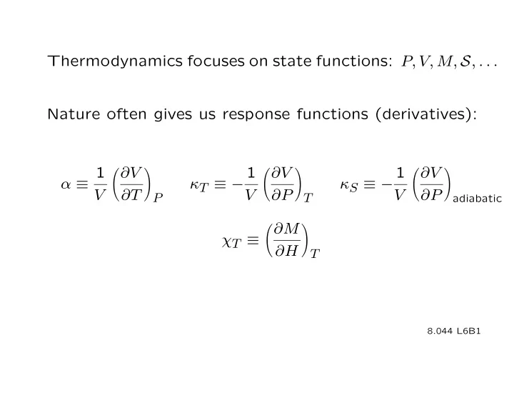
Thermodynamics focuses on state functions: P, V, M, S, . . . Nature often gives us response functions (derivatives): 1

∂V

  • 1

∂V

  • 1

∂V

  • α ≡ V

∂T P κT ≡ − V ∂P T κS ≡ − V ∂P adiabatic

  • ∂M

χT ≡ ∂H T

8.044 L6B1

slide-2
SLIDE 2

Example Non-ideal gas Given

  • Gas → ideal gas for large T & V
  • ∂P

Nk

  • =

∂T

V

V − Nb

  • ∂P

NkT 2aN2

  • = −

+ ∂V

T

(V − Nb)2 V 3 Find P

8.044 L6B2

slide-3
SLIDE 3

dP =

  • ∂P

∂V T dV +

  • ∂P

∂T V dT P =

  • ∂P

∂T V dT + f(V ) =

  • Nk

V − Nb dT + f(V ) = NkT (V − Nb) + f(V )

8.044 L6B3

slide-4
SLIDE 4
  • ∂P

NkT NkT 2aN2 = − + fI(V = − + ∂V (V − Nb)2

j V ) )

(V − Nb)2 V 3

T

j ) V

2aN2 aN2 f(V ) = dV = − + c V 3 V 2 NkT aN2 P = − + c (V − Nb) V 2 but c = 0 since P → NkT/V as V → ∞

8.044 L6B4

slide-5
SLIDE 5

Internal Energy U Observational fact

final

∆W

initial isolated (adiabatic)

Final state is independent of how ∆W is applied. Final state is independent of which adiabatic path is followed.

8.044 L6B5

slide-6
SLIDE 6

⇒ a state function U such that ∆U = ∆Wadiabatic U = U(independent variables) = U(T, V ) or U(T, P ) or U(P, V ) for a simple fluid

8.044 L6B6

slide-7
SLIDE 7

Heat If the path is not adiabatic, dU /W = d d /Q ≡ dU − d /W d /Q is the heat added to the system. It has all the properties expected of heat.

8.044 L6B7

slide-8
SLIDE 8

First Law of Thermodynamics dU = d /Q + d /W

  • U is a state function
  • Heat is a flow of energy
  • Energy is conserved

8.044 L6B8

slide-9
SLIDE 9

Ordering of temperatures

T1 T2

dQ

When d /W = 0, heat flows from high T to low T.

8.044 L6B9

slide-10
SLIDE 10

Example Hydrostatic System: gas, liquid or simple solid Variables (with N fixed): P, V, T, U. Only 2 are independent.

   

d /Q d /Q

   

CV ≡ CP ≡ dT dT

V P

Examine these heat capacities.

8.044 L6B10

slide-11
SLIDE 11
  • dU = d

/Q + d /W = d /Q − P dV d /Q = dU + P dV d We want . We have dV . dT ∂U ∂U dU = dT + dV ∂T V ∂V T

8.044 L6B11

slide-12
SLIDE 12
  • ∂U

∂U d /Q = dT + + P dV ∂T V ∂V T

  • d

/Q ∂U ∂U dV ⇒ = + + P dT ∂T V ∂V T dT

⎛ ⎞

d /Q ∂U CV ≡ ⎝

= dT ∂T V

V

8.044 L6B12

slide-13
SLIDE 13

  • d

/Q ∂U ∂U ∂V CP ≡ ⎝

= + + P dT ∂T V ∂V T ∂T P

P

" T v " T v

CV αV

∂U CP − CV = + P αV ∂V T The 2nd law will allow us to simplify this further. ∂U Note that CP . = ∂T P

8.044 L6B13

slide-14
SLIDE 14

∆ ∆ ∆

8.044 L6B14

slide-15
SLIDE 15

  • ρ
  • ρκ

8.044 L6B15

slide-16
SLIDE 16
  • ∂U

∂V

  • T

= 0

8.044 L6B16

slide-17
SLIDE 17

No work done so ∆W = 0 Tf = Ti ⇒ ∆Q = 0 together ⇒ ∆U = 0 → (∂U/∂V )T = 0

, U= Q , U= Q

here quasi-static changes

  • Physics: no interactions, single particle energies
  • nly ⇒ (∂U/∂V )T = 0
  • Thermo: 2nd law + (PV = NkT ) ⇒ (∂U/∂V )T = 0

8.044 L6B17

slide-18
SLIDE 18
  • Consequences

∂U ∂U dU = dT + dV ∂T V ∂V T

j V ) j V )

CV T

U = CV (T ') dT ' + constant

j V )

set=0 In a monatomic gas one observes CV = 2

3Nk.

Then the above result gives U = CV T = 2

3NkT .

8.044 L6B18

slide-19
SLIDE 19
  • ∂U

∂V CP − CV = ( +P ) ∂V ∂T

,

T

p ,

P

p

∂ ∂T (NkT/P )P =Nk/P

= Nk for any ideal gas Applying this to the monatomic gas one finds 3 5 CP = Nk + Nk = Nk 2 2 5 γ ≡ CP /CV = 3

8.044 L6B19

slide-20
SLIDE 20
  • Adiabatic Changes

d /Q = 0 Find the equation for the path. Consider a hydrostatic example.

  • ∂U

∂U d /Q = dT + + P dV = 0 ∂T V ∂V T

" T v " T v

CV (CP −CV )/αV

⎛ ⎞

∂T CP − CV ) 1 (γ − 1)

⎝ ⎠

= − = − ∂V ∆Q=0 CV αV αV This constraint defines the path.

8.044 L6B20

slide-21
SLIDE 21

Apply this relation to an ideal gas. 1

∂V

  • 1 ∂

NkT

  • 1

Nk

  • 1 V

1 α ≡ = = = = V ∂T P V ∂T P

P

V P V T T Path dT T = −(γ − 1) dV V

⎛ ⎞

dT dV T V

⎝ ⎠

= −(γ − 1) → ln = −(γ − 1) ln T V T0 V0

⎛ ⎞ ⎛ ⎞−(γ−1)

T V

⎝ ⎠ ⎝ ⎠

= T0 V0

8.044 L6B21

slide-22
SLIDE 22

Adiabatic TV γ−

1 = c "

PV γ = c γ = 5/3 (monatomic) V −

5/3

P ∝ dP 5 P = − dV 3V

c)

  • Isothermal

""

PV = c V −

1

P ∝ dP P = − dV V

8.044 L6B22

slide-23
SLIDE 23

  • 8.044 L6B23
slide-24
SLIDE 24

Starting with a few known facts, 1st law, d /W , and state function math,

  • ne can find

relations between some thermodynamic quantities, a general expression for dU, and the adiabatic constraint. Adding models for the equation of state and the heat capacity allows one to find the internal energy U and the adiabatic path.

8.044 L6B24

slide-25
SLIDE 25

MIT OpenCourseWare http://ocw.mit.edu

8.044 Statistical Physics I

Spring 2013 For information about citing these materials or our Terms of Use, visit: http://ocw.mit.edu/terms.