
SLIDE 1
Today’s Discussion
To date:
- Neural networks: what are they
- Backpropagation: efficient gradient computation
- Advanced training: conjugate gradient
Today:
- CG postscript: scaled conjugate gradients
- Adaptive architectures
- My favorite neural network learning environment
- Some applications
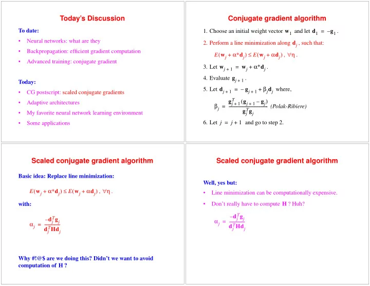
Conjugate gradient algorithm
- 1. Choose an initial weight vector
and let .
- 2. Perform a line minimization along
, such that: , .
- 3. Let
.
- 4. Evaluate
.
- 5. Let
where, (Polak-Ribiere)
- 6. Let
and go to step 2. w1 d1 g1 – = dj E wj α∗dj + ( ) E wj αdj + ( ) ≤ η ∀ wj
1 +
wj α∗dj + = gj
1 +
dj
1 +
gj
1 +
– βjdj + = βj gj
1 + T
gj
1 +
gj – ( ) gj
Tgj
- =
j j 1 + =
Scaled conjugate gradient algorithm
Basic idea: Replace line minimization: , . with: Why #!@$ are we doing this? Didn’t we want to avoid computation of ? E wj α∗dj + ( ) E wj αdj + ( ) ≤ η ∀ αj dj
Tgj
– dj
THdj
- =
H
Scaled conjugate gradient algorithm
Well, yes but:
- Line minimization can be computationally expensive.
- Don’t really have to compute
? Huh? H αj dj
Tgj
– dj
THdj
- =