Using Physics-Like Interaction Law to perform Active Environment - - PDF document

1

Using Physics-Like Interaction Law to perform Active Environment Recognition in Mobile Robotics

• A. Hazan, F. Davesne, V. Vigneron, H. Maaref

Laboratoire Syst` emes Complexes (LSC), CNRS FRE 2494 CE 1433 Courcouronnes 40, Rue du Pelvoux 91020 Evry Cedex Phone: +0033169477504, E-mail: {hazan,davesne,vvigne,maaref}@iup.univ-evry.fr

Abstract - In this article, we give some insights of a novel method for active environment recognition in mobile robotics. The basic idea consists on utilizing a Physics-like interac- tion law to fix a relation between sensors and effectors val- ues at any time. Our main assumption is that the trajectory

• f the robot in the phase space, which depends uniquely on

its environment -when the law and the nature of the robot are fixed- may discriminate environments better than classi- cal Data Analysis Approaches (DAA). In order to test our as- sumption, we choose to model an analogical robot which light sensor amplitudes and wheels speed are coupled in a set of differential equations. As a result, we show that our Interac- tionist Approach (IA) is tractable and perform well for dis- criminating simple environments, comparing to a data analy- sis (DA) strategy. Keywords— Mobile Robotics, Dynamic Systems, Environe- ment Recognition, Physics-like interaction

• I. INTRODUCTION
• A. Framework

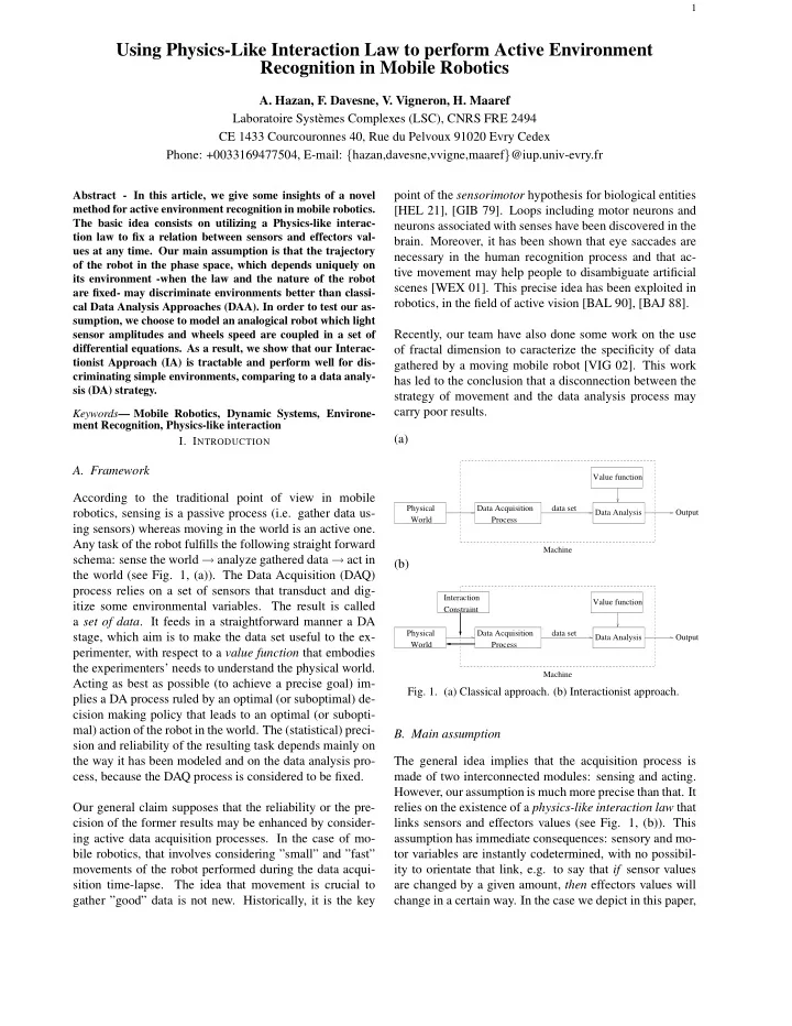
According to the traditional point of view in mobile robotics, sensing is a passive process (i.e. gather data us- ing sensors) whereas moving in the world is an active one. Any task of the robot fulfills the following straight forward schema: sense the world → analyze gathered data → act in the world (see Fig. 1, (a)). The Data Acquisition (DAQ) process relies on a set of sensors that transduct and dig- itize some environmental variables. The result is called a set of data. It feeds in a straightforward manner a DA stage, which aim is to make the data set useful to the ex- perimenter, with respect to a value function that embodies the experimenters’ needs to understand the physical world. Acting as best as possible (to achieve a precise goal) im- plies a DA process ruled by an optimal (or suboptimal) de- cision making policy that leads to an optimal (or subopti- mal) action of the robot in the world. The (statistical) preci- sion and reliability of the resulting task depends mainly on the way it has been modeled and on the data analysis pro- cess, because the DAQ process is considered to be fixed. Our general claim supposes that the reliability or the pre- cision of the former results may be enhanced by consider- ing active data acquisition processes. In the case of mo- bile robotics, that involves considering ”small” and ”fast” movements of the robot performed during the data acqui- sition time-lapse. The idea that movement is crucial to gather ”good” data is not new. Historically, it is the key point of the sensorimotor hypothesis for biological entities [HEL 21], [GIB 79]. Loops including motor neurons and neurons associated with senses have been discovered in the

• brain. Moreover, it has been shown that eye saccades are

necessary in the human recognition process and that ac- tive movement may help people to disambiguate artificial scenes [WEX 01]. This precise idea has been exploited in robotics, in the field of active vision [BAL 90], [BAJ 88]. Recently, our team have also done some work on the use

• f fractal dimension to caracterize the specificity of data

gathered by a moving mobile robot [VIG 02]. This work has led to the conclusion that a disconnection between the strategy of movement and the data analysis process may carry poor results. (a)

Physical World Data Analysis Value function Output Machine data set Process Data Acquisition

(b)

Physical World Data Analysis Value function Interaction Constraint Output Machine data set Process Data Acquisition

• Fig. 1. (a) Classical approach. (b) Interactionist approach.
• B. Main assumption

The general idea implies that the acquisition process is made of two interconnected modules: sensing and acting. However, our assumption is much more precise than that. It relies on the existence of a physics-like interaction law that links sensors and effectors values (see Fig. 1, (b)). This assumption has immediate consequences: sensory and mo- tor variables are instantly codetermined, with no possibil- ity to orientate that link, e.g. to say that if sensor values are changed by a given amount, then effectors values will change in a certain way. In the case we depict in this paper,

the sensory motor law is modeled by a set of coupled differ- ential equations. The solutions (when then exist) are trajec- tories in the phase space (combining sensors and effectors variables). The class of solutions may be interpreted as the set of all possible behaviors of the robot facing all possible

• worlds. A particular trajectory in the phase space is deter-

mined during the experiment, when the robot is facing a particular world. Thus, two different trajectories (given a certain distance) may be associated to two different envi- ronments (see Fig. 2) : this determines the basic principle for an environment recognition process.

X X

1 2

possible environments

• Fig. 2. Different trajectories associated to different environments.

X1 and X2 are the variables of the phase space. We depict two planes over the environment axis, representing two dif- ferent environments. The different trajectories in the same plane represent different behaviors of the robot placed in dis- tinct areas of the same environment.

The existence of a physics-like interaction law is a strong constraint because the relation between sensory motor vari- ables must be fulfilled at any time. It is based on an ac- tion/reaction procedure: the world (which is a priori un- known) acts on the robot by the way of the sensor values and the movement of the robot and, at the same time, the machine reacts to adapt its internal parameters (which are known) in order to follow the interaction law. This ac- tion/reaction procedure has already been successfully uti- lized to design a reinforcement learning algorithm onto which convergence proofs may easily be given [DAV 99], [DAV 04]. One particular advantage consists on the possi- bility to determine the class of solutions before the exper-

• iment. In our case, this permits to have an idea about the

similarity of the shapes of the possible trajectories. The more two shapes are ”different”, the easiest it is to discrim- inate the two associated environments.

• C. Environment recognition - interactionist versus classi-

cal approach In this article we focus on an environment recognition task in which recognition is made by gathering data over a fixed time-lapse d. In a general sense, that means that the robot first evolves locally in a given target environment, following some trajectory we will discuss later in this pa-

• per. Then, it is presented to a series of k distractive envi-

ronments (i.e. that may or may not correspond to the target environment) where it evolves during d as in the first stage. The aim of this task consists on identifying the target en- vironment among the distractive environments on the basis

• f the data collected and analyzed during the various ex-

periments. In the classical approach, called DA Approach (DAA), this implies to put the robot in two given environments, to ex- ecute the same trajectory in both cases and to compare the corresponding sensor values. The discrimination between two environments is then given by a distance between two sensor data vectors. In our approach, called Interactionist Approach (IA), the robot moves in order to fulfill the interaction law. And its motion during the time-lapse d depends on the sensor values, hence the environment. So, one cannot force the robot’s trajectory over d, but one may hope that this tra- jectory is a signature of a local robot/environment interac-

• tion. The discrimination between two environments is then

given by a distance between two trajectories in the phase space combining sensor and effector variables.

• D. Issues covered by this paper

We have chosen to model the interaction law with a set of coupled differential equations, which is a particular way

• f implementing our assumption. In this paper, we detail

issues arising from this choice and provide simple exam- ples in which artificial worlds may be discriminated by a simulated robot after using our approach and compared to the classical approach. These results are the beginning of a work leading to an extended comparison, both theoretical and experimental, between the results obtained by the clas- sical approach and ours.

• II. MODELIZATION OF OUR ASSUMPTION
• A. General Principle for discriminating environments in

the IA approach In IA, we impose a local discrimination criterion on the Data Acquisition stage. To make it clearer, we assume that the Data Acquisition step defines a multidimensional phase space that includes both motor and sensitive data, in which a state is called X. The interaction of the robot is thus rep- resented in this space by a trajectory T : t → X(t). We then suppose that the robot can take two simultaneous dif- ferent - but “close” - interactive measures, i.e. that it can follow at the same time two different but close trajectories T1 and T2 of the phase portrait. We also assume that the in- teraction is not a completely deterministic process, but that it has a stochastic component. We may then think of two

realizations of the same stochastic process, represented by two trajectories T1 and T

′

1.

We state that the robot is able to discriminate locally be- tween sensorimotor trajectories if we can exhibit a distance function operating on trajectories (T1, T2) → T1, T2, such that the following constraint C1 if fulfilled: C1 : T1, T2 > T1, T

′

1

Roughly, it means that two trajectories (produced by the interaction with two environments) must be more different (in the sense of a distance to be defined) than two realiza- tions of the same trajectory (produced by the interaction with one environment). The issue is that the robot have to interact at the same time along two different trajectories. To comply with this requirement, while avoiding to inter- rupt the interaction, we imagine to make the DAQ stage both able to:

• apply a discontinuous perturbation at some given instant
• f its interaction along trajectory T1.
• predict the lacking semi-trajectories that would have oc-

curred if no perturbation had happened.

• Fig. 3 illustrates this idea. Note that we thus constrain the

notion of locality, both in the spatial sense (proximity be- tween sensorimotor trajectories in the phase space, accord- ing to a distance) and temporal sense (time span required to make two trajectories out of one). Locality extends to the distance functions, since we don’t define a global distance, but instead functions that locally verify the constraint (C1). X X

1 2

δ

• Fig. 3. Perturbation and prediction to make two trajectories out of
• ne. Thick lines are measured interactions, dashed lines are

predicted ones. Zigzag curve marked with δ is the perturba-

• tion. Other curves form the phase portrait in the sensorimotor

phase space (X1, X2).

• B. Model of the robot’s interaction with its environment

First, we discuss the formalism in which to express the interaction of the robot in its environment. Because we need a balanced representation that takes into account sen- sitive and motor values at the same time, in a deterministic fashion, we favor the Theory of Dynamical Systems as our main theoretical framework. The physical variables that determine the robot’s behavior submit to a system of dif- ferential equations that involve the internal variables of the robot Xi (value returned by the sensors, current that feeds the motors, rotation speed of the wheels) and the external variables Xe (position in the environment). This system is coupled to another one that links the absolute position of the robot in the environment to the value returned by its

• sensors. As an example, we present the coupling dynamics

˙ Xi = AXi + f(Xe) (1) ˙ Xe = g(Xe, Xi) (2) When it exists, we note T : t → (Xi(t), Xe(t)) a solution

• f this system. The trajectories T1 and T2 are projections
• f such solution in the space of internal variables. Indeed,

we impose that the robot ignores the value of the external variables to which it has no access. The internal variables are the only one it can be aware of. Hence, the mentioned trajectories are the projections Ti : t → Xi(t) of the gen- eral solutions on the space of internal variables, and will be used by both DAA and IA. The DAQ step generally needs sensors to be chosen -that fit specific physical variables- and placed in such a way that meaningful measures (in the sense of the experimenter) can be taken. This may include an appropriate setting of the position and speed of the sensors in the 3D space. For that purpose, the robot is equipped with effectors that enable it to move across the environment. The DA step often per- forms a discretization (i.e. sampling and quantization) and some projection from the temporal domain to the frequen- tial one (e.g. Fourier transform, wavelet analysis). Both participate to the creation of a phase space, associated with some ad hoc function endowed with the properties of a dis-

• tance. The aim of this space is to give a “complete descrip-

tion” of the observed environment; which means that any two environments that the experimenter can distinguish are separate in the metric phase space. Let’s sum up the main steps performed during DA and DAQ stages:

• choice of physical continuous variables measured by

sensors, including their respective positions and speeds.

• choice of a phase space via discretization, projection and

filtering.

• choice of a distance on the phase space.

The value function evoked in section II, imposed by the ex- perimenter, has to maintain an analogical link between the

complexity of the DA step -in an algorithmic sense- and the discriminability of two environments for the experimenter. To give an intuitive feeling of this idea, let’s imagine a cou- ple of environments E1 and E2 that are obviously distinct in the experimenter’s perception, and another couple E3 and E4 that are almost the same in the same sense. Then the DA step needed to distinguish the two environments

• f the first couple must be less complex than in the sec-
• nd case, algorithmically speaking. Note that DAA and IA

share this analogical constraint as a value function. Now let’s focus on the instantiation of the Interaction con- straint acting on the DAQ stage evoked in subsection II-A. (C1) is verified if and only if there exists a distance func- tion operating on trajectories (T1, T2) → T1, T2, such that T1, T2 > T1, T

′

1.

To be able to verify it, the robot must compute T1, T ′

1 and T1, T2. The first one

requires the system to interact twice along the same sen- sorimotor trajectory, while the second needs two neighbor- ing trajectories, with respect to a given distance. As we already stated, we introduce a twofold procedural mecha- nism, named Local Discrimination Criterion that enforces these conditions without interrupting the interaction: on

• ne hand, we apply a cyclic discontinuous perturbation on

the system’s dynamics so as to leap from one trajectory to another. On the other hand, we assume that the sys- tem is endowed with a model of its own interaction with the environment that allows it to give predictions on future

• r past trajectories. Consequently, after the perturbation

has occurred, the interaction goes on and finally the robot gets two half-trajectories. At this point, it uses its predictor to extrapolate the future trajectory, that would have took place if no perturbation had occurred, as well as the past

• f the actual trajectory, if time could reverse. Note first,

that this mechanism can also be used to estimate a realiza- tion T

′

1 of an ongoing trajectory, given its initial condition.

• Fig. 4 summarizes these ideas. Secondly we remark that

unlike the robot/environment interaction where each part influences instantly the other in a symmetric way, the na- ture of the influence of the perturbating mechanism on the dynamics is sequential: first, the perturbation takes places while the robot/environment interaction goes on, then the corresponding recorded data is processed to check the va- lidity of (C1). Finally, we suggest that the perturbation δX itself may be applied incrementally: if, once triggered, it doesn’t allow criterion (C1) to be verified, then the intensity of the per- turbation is increased next time, and so on until either (C1) is verified, or a threshold is reached, which allows the robot to conclude that (C1) can’t be verified in that configuration (both of the robot, the environment, and the system of dif- ferential equations modeling the interaction).

• C. Implementation

In this part we discuss more technically a possible imple- mentation of the mobile robot that illustrates the measure-

Two realisations

• f a trajectory

Xi=... . Xe=... .

Model Internal Half−trajectory Measure Xi=... . Xe=... . Half trajectory Completion Environment Perturbation Measure Machine Local discrimination criterion (C1)

• Fig. 4. Inner structure of the machine, where the local discrimi-

nation criterion (C1) influences the machine/environment in- teraction.

ment process seen in the beginning of this section, and ap- plied to the context of robotics as in section II-B, before in- stantiating the recognition algorithm in the compared cases. C.1 Analogical modelization of the robot All the experiments conducted in this article are simulated because, mainly, we consider an analogical robot which ac- tive sensors do not exist in reality. The manipulated differ- ential equation systems, will be solved numerically with LSODE 1 . The environment is assimilated to a light-emitting curve whose shape is a circle. In every point M(x, y) of the phys- ical space, one can then measure the intensity of incoming light radiations. The function I(x, y) plotted in figure 5 depicts that intensity landscape.

10 20 30 40 50 60 x 10 20 30 40 50 60 y 2 4 6 8 10

• Fig. 5. Voltage returned by light sensors as a function of (x, y).

1 Livermore

Solver for Ordinary Differential Equations http://www.netlib.org/odepack/opkd-sum

The robot is equipped with two continuous current motors

• n the left and right, fed by currents il and ir. Two light

sensitive diodes (FLEDs) are connected to an intermediary level that couples the two sides of the robot in a way such that the voltages and currents feeding both motors depend

• n the voltage produced by both diodes. Fig. 6 summarizes

those facts. The motors are linked to wheels whose angu- lar velocity are noted (ωl, ωr), and that enable the robot to move on a planar surface.

x A

M M

x B x B

Σ Σ

x A

u u

ω ω i i

l

r r r

l l

• Fig. 6. Electrical circuit governing the robot’s behavior

We do not exhibit precisely the modeling process lead- ing to the equations shown in section II-B that account for the robot/environment interaction. We will develop them below. First notice than Xi = [wl, il, wr, ir]T while Xe = [x, y, θ]T, where x and y stand for the absolute posi- tion of the center of the robot, while θ stands for its orien- tation with respect to some fixed direction. Now equations 1 in a developed form may be written as follows:                            ˙ Xi =AXi + f(Xe) f(Xe)=[0 ul 0 ur ]T ul =U0 + αvl + βvr ur =U0 + βvr + αvl vl/r =V0

• e−

rl/r−ro

σ

2 rl/r =

• x2

l/r + y2 l/r

xl/r =x + e cos(θ ∓ π/2) yl/r =y + e sin(θ ∓ π/2) Similarly, we develop equation 2    ˙ x=d/2 (ωl cos θ + ωr cos θ) ˙ y=d/2 (ωl sin θ + ωr sin θ) ˙ θ= d

2e(−ωl + ωr)

Note that both f and g in equations 1 and 2 are highly non- linear, what makes it hard to find an analytic solution to the system. We then focus on the predictor we proposed in subsec- tion II-B. Remember it is necessary to extrapolate inter- rupted trajectories in the future and in the past. We could choose a classical time-series method relying for example

• n Kalman filtering but instead we endow the machine with

an inner numerical integration method, as well as an ap- proximate differential equation system. Doing so, giving the initial condition XO

i allows the system to predict a full

trajectory in the future of in the past. C.2 Recognition Algorithm So far we’ve described the robot, the environment, and their interaction law. However we lack a precise formalization

• f the environment recognition algorithm itself. In both

classical or interactive perspective, each comparison needs two experiments, with the same mobile robot but different environments, in addition to an identity operator. In the classical case, the robot is placed in the environment and moves in it. For the sake of comparison, we focus on the discrete sequence of internal variables T : tk → Xi(tk)

• btained with the interactionist method. The outputs O1

and O2 thus produced are two matrices T1 and T2. One has to build a distance ., . on the space of such matrices, as well as a threshold ε. Classically any couple of environ- ments which corresponding matrices verify T1, T2 ≤ ε will be considered identical. This algorithm is illustrated by Fig. 7 (a). The output, returned by the corresponding set of experi- ments in the interactionist case, is a little more intricate. It first includes the discretized internal trajectories T : tk → Xi(tk). Remind that we perturbate the interaction in a cyclic manner. This process naturally delimitates seg- ments of the internal variables trajectories. Secondly, each segment comes with a -possibly empty- set of distances {., .i}i=1..n that verify the Local Discrimination Crite-

• rion. Let us focus on this local level: for each segment,

we compare the sets of C1-complying distance functions, corresponding respectively to the first and second experi-

• ments. If for a given couple of corresponding 2 segments

(S1,k, S2,k), the C1-complying distance set is nonempty, we can compare those distances. If we can find the same distance in both sets, we call this distance a compatible one. If, according to that distance, the (C1) criterion is verified (i.e. S1,k, S2,k > S1,k, S′

1,k), then the segments are

distinct, and so are the two global trajectories. If for all seg- ments k, we find a nonempty distance set, among which we exhibit a compatible distance, according to which the seg- ments are undiscriminable, then the trajectories are identi-

• cal. This is summarized in Fig. 7 (b).

2 that notion of correspondence -in a discrete framework- implies that the

perturbation frequency as well as the sampling frequency are identical in both experiments

(a)

Machine Machine Environment 1 Envionment 2 Experiment 1 Experiment 2 O1=T1 O2=T2 ? <.,.> < ε identity

(b) Machine Machine C1 existence compatibility ?

i

O1=(T1,{<.,.> }) Environment 1 Envionment 2 Experiment 1 Experiment 2

• Fig. 7. Environment recognition in a classical (a) and interactive

(b) perspective.

• III. RESULTS

In the previous section, we’ve detailed the comparison pro- tocol between DAA and IA. Now we present some re- sults for the environment recognition process. As we al- ready said, we place the robot in a target environment E0 where it obeys the aforementioned interaction process. Then we place it in three other environments E1, E2, E3 where E2 = E0, and all the others are distinct as shown by Fig. 8. The associated local trajectories in a projection space made of internal variables only are presented in Fig. 9 (we note that T0 and T2 are not superposed, because of the stochastic nature of the interaction).

• A. The IA case

In that case, we obtain both a trajectory T0 in the space

• f internal variables Xi, and a set of distances {., .}0

that verify criterion (C1). Then we start again in k dis- tractive environments and we similarly obtain k trajecto- ries Ti=1...k. Each trajectory also comes with a potentially

10 20 30 40 50 60 0 10 20 30 40 50 60

E1 E2 E3 E0,

• Fig. 8. Environments (E0, E1, E2, E3).

empty set of distance functions {., .}i. Here, if we note Ti and Tj two trajectory matrices, the possible distances we use are associated with the built-in norms in Octave 3 :

• Ti, Tj1: the largest column sum of the absolute values
• f Ti − Tj.
• Ti, Tj2: largest singular value of Ti − Tj.
• Ti, Tj3: infinity norm, the largest row sum of the abso-

lute values of Ti − Tj.

• Ti, Tj4:

Frobenius norm

• f

Ti − Tj, i.e.

• ( (diag((Ti − Tj)′ ∗ (Ti − Tj)))).

Then, according to the method previously exposed, we be- gin by verifying that all trajectory come with a nonempty set of C1-complying distance functions. Table I shows that trajectories T0, T2, T3 satisfy that constraint (which is marked by an ’x’). Furthermore, we remark that the con- cerned distances are all compatible. Hence, we can com- pare T0 with T2 and T3 with distances ., .k=1,2,3,4. The last step is to verify -only for environments that passed the previous test- the (C1) criterion, i.e. Ti, Tjk < Ti, T ′

ik,

which means that Ti and Tj can’t be distinguished from the point of view of ., .k. Table II gives, for each cou- ple Ei, Ej and for each distance ., .k, the result under the form a/b where a = Ti, Tjk and b = Ti, T ′

• ik. The

result is highlighted when a < b, i.e. when the correspond- ing environments can’t be distinguished with the associated

• distance. We observe that T0 and T3 are distinct for all dis-

tances, consequently E0 and E3 are different from an inter- actionist point of view. However, T0 and T2 are equal for distances ., .1, ., .3, ., .4. As a result we can state that this method has succeeded in identifying E0 and E2, while the others were discarded.

3 GNU Octave is a numerical computation language, available under

GNU General Public License (GPL) http://www.octave.org/

TABLE I C1-COMPLYING DISTANCES FOR EACH ENVIRONMENT

Environment Distances ., .1 ., .2 ., .3 ., .4 E0 x x x x E1

• E2

x x x x E3 x x x x

TABLE II TRAJECTORY COMPARISON IN IA

Trajectory Distances ., .1 ., .2 ., .3 ., .4 (T0, T2) 93/104 4/3 0.3/0.9 4/8 (T0, T3) 5381/104 284/3 29/0.9 284/8

• B. The DAA case

In this case, we only obtain a trajectory T0 in the inter- nal variables space, as well as k trajectories Ti=1...k corre- sponding to the distractive environments. Table III presents values of Ti, Tjk for the different distances depicted

• above. Unless we fix a threshold for each distance this ta-

ble is useless. Once it is fixed, one may state that, for a given distance, Ti and Tj are equivalent and consequently Ei and Ej are equivalent too. For example, if we impose the same threshold ε = 3.5 for all distances, T0 and T1 are equal according to distance ., .3 -although they were generated by interactions in dif-

• 0.5

0.5 1 1.5 2 2.5 3 3.5 4

• 0.1

0.1 0.2 0.3 0.4 0.5 0.6 0.7 0.8 intensity (i) angular velocity (w)

E3 E0 E1 E2

• Fig. 9.

Internal trajectory t → (wr(t), ir(t)) in different envi- ronments (E0, E1, E2, E3). TABLE III TRAJECTORY COMPARISON IN DAA

Trajectory Distances ., .1 ., .2 ., .3 ., .4 (T0, T1) 389 22 3 22 (T0, T2) 93 4 0.3 4 (T0, T3) 5381 284 29 284

ferent places- as well as T0 and T2, while T0 and T3 are dif- ferent for all distances. We could also impose a distance- depending threshold ε = [ε1 ε2 ε3 ε4], but the arbitrary nature of this choice remains the same.

• C. Conclusion

In DAA, one may compute several distances between tra- jectories, but has to fix a threshold in order to conclude to the indiscriminability of two environments given a per- formed trajectory. As we saw, the mere choice of this threshold, be it differentiated with respect to the considered distance, yields the recognition result. On the opposite, the interactionist approach returns a set

• f (C1) relevant distances for every trajectory. If none is

provided, no comparison is possible, thus discrimination is impossible. If not, two trajectories may be compared with respect to that distance that has a local discrimination capability. We can’t deny that the IA approach makes specific as- sumptions, namely that discrimination is conditionned by the compliance towards criterion (C1). Furthermore, we create a priori the set of possible distance functions, the trajectory duration, the sampling frequency as well as the composition of the phase space, but these are not distinc- tive features of the IA method and are intrinsic drawbacks when simulating a physical phneomenon on a digital com-

• puter. All things considered, it seems to us that criterion

(C1) is less arbitrary than imposing both the distance and the threshold.

• IV. CONCLUSION AND FUTURE WORK

In this article, our aim was to confront a balanced con- ception of robot/environment interaction, with the passive way in which a robot classically performs discrimination and recognition tasks. To ensure a Physics-like interaction between sensors and effectors values at any time, we’ve adopted the theoretical framework of the Dynamical Sys- tems Theory so as to model an analogical robot which sen- sors and motors values are coupled via a set of differential

• equations. Furthermore, adding a discrimination constraint
• n the robot/environment interaction, and focusing on sen-

sorimotor trajectories rather on sensory data only, we show that our method makes it possible both to know whether the robot can discriminate or not, then to actually discrim- inate several types on interaction if discrimination has a

• sense. Finally we show that this can be used to recognize

an environment if the interaction is performed in the same conditions, in a way comparable to the classical approach, where one can discriminate sensory or motor trajectories, given some metric constraints and the choice of a thresh-

• ld.

Let us now consider the perspectives opened by this work. 1) developping this framework could be achieved in sev- eral ways:

• verifying the invariance of recognition towards spatial

transformation.

• implementing a real analog robot instead of simulating

it.

• implementing an analog architecture of the Local Di-

crimination Criterion since the current version is based

• n a discrete method. Reasons for this choice are dis-

cussed in the field of epistemology by [BAI 04]. 2) criticizing this framework draws the following topics to be questionned:

• why describing the discrimination capability in a metric

framework, even if the distance can be changed during the experiment ?

• why keeping the robot, its interaction law and the

environnement unchangeable ? Exploring their pos- sible codetermination needs to make them deformable (e.g. non-rigid robot morphology, non-rigid environ- ment, “deformable” differential equation system).

• why choosing the Dynamical Systems Theory frame-

wok that lacks that idea of deformable phase space ?

REFERENCES [BAI 04] BAILLY F., LONGO G., Causalit´ es et sym´ etries dans les Sciences de la Nature. Le Continu et le Discret Math´ ematiques, Logique et Interaction, Joinet, 2004. [BAJ 88] BAJCSY R., Active Perception, Special Issue on Com- puter Vision, vol. 76,8, IEEE, August 1988. [BAL 90] BALLARD D., Animate Vision, Artificial Intelligence,

• p. 57–86, 1990.

[DAV 99] DAVESNE F., BARRET C., Reactive navigation of a mobile robot using a hierarchical set of learning agents, Conf. on Robotics and autonomous Systems IROS’99, vol. 1, IEEE/RJS,

• p. 482–487, 17-21 oct 1999.

[DAV 04] DAVESNE F., Learning from Reward as an emergent property of Physics-like interactions between neurons in an arti- ficial neural network, ESANN’04, IEEE, p. 537–542, 28-30 apr. 2004. [GIB 79] GIBSON J., The ecological approach to visual percep- tion, Hillsdale, 1979. [HEL 21] HELMHOLTZ H., Epistemological writings, The P. Hertz M. Schlick Centenary Edition, 1921. [VIG 02] VIGNERON V., DAVESNE F., MULLER A., Reconnais- sance dynamique d’environnements par un robot mobile Khepera, NSI’02, 2002. [WEX 01] WEXLER M., PANERAI F., LAMOURET I., DROULEZ J., Self-motion and the perception of stationary objects, Nature, vol. 409, p. 85–88, 4 Jan. 2001.