Using Uncertain Knowledge Agents dont have complete knowledge about - - PowerPoint PPT Presentation

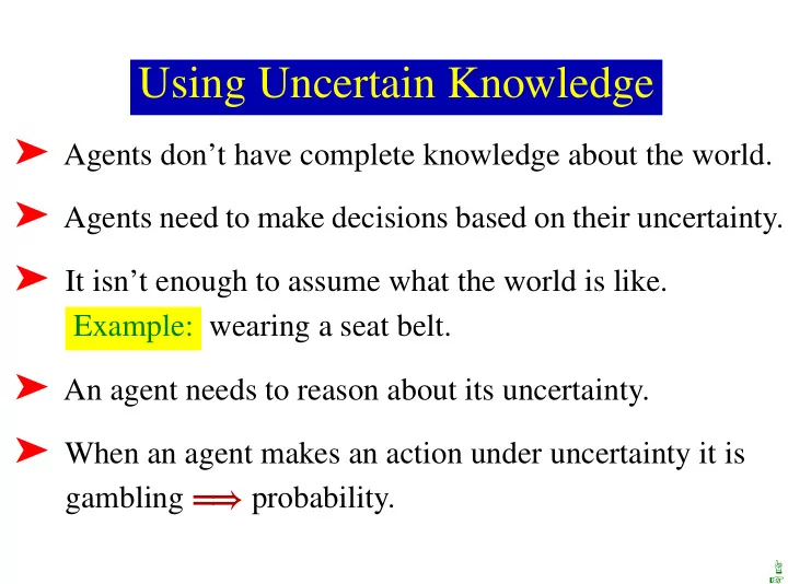
Using Uncertain Knowledge

➤ Agents don’t have complete knowledge about the world. ➤ Agents need to make decisions based on their uncertainty. ➤ It isn’t enough to assume what the world is like.

Example: wearing a seat belt.

➤ An agent needs to reason about its uncertainty. ➤ When an agent makes an action under uncertainty it is

gambling ⇒ probability.

☞ ☞

Probability

➤ Probability is an agent’s measure of belief in some

proposition — subjective probability.

➤ Example: Your probability of a bird flying is your

measure of belief in the flying ability of an individual based only on the knowledge that the individual is a bird.

➣ Other agents may have different probabilities, as they

may have had different experiences with birds or different knowledge about this particular bird.

➣ An agent’s belief in a bird’s flying ability is affected

by what the agent knows about that bird.

☞ ☞ ☞

Numerical Measures of Belief

➤ Belief in proposition, f , can be measured in terms of a

number between 0 and 1 — this is the probability of f .

➣ The probability f is 0 means that f is believed to be

definitely false.

➣ The probability f is 1 means that f is believed to be

definitely true.

➤ Using 0 and 1 is purely a convention. ➤ f has a probability between 0 and 1, doesn’t mean f is

true to some degree, but means you are ignorant of its truth value. Probability is a measure of your ignorance.

☞ ☞ ☞

Random Variables

➤ A random variable is a term in a language that can take

• ne of a number of different values.

➤ The domain of a variable X, written dom(X), is the set

• f values X can take.

➤ A tuple of random variables X1, . . . , Xn is a complex

random variable with domain dom(X1) × · · · × dom(Xn). Often the tuple is written as X1, . . . , Xn.

➤ Assignment X = x means variable X has value x. ➤ A proposition is a Boolean formula made from

assignments of values to variables.

☞ ☞ ☞

Possible World Semantics

➤ A possible world specifies an assignment of one value

to each random variable.

➤ w |

= X = x means variable X is assigned value x in world w.

➤ Logical connectives have their standard meaning:

w | = α ∧ β if w | = α and w | = β w | = α ∨ β if w | = α or w | = β w | = ¬α if w | = α

➤ Let be the set of all possible worlds.

☞ ☞ ☞

Semantics of Probability: finite case

For a finite number of possible worlds:

➤ Define a nonnegative measure µ(w) to each set of worlds

w so that the measures of the possible worlds sum to 1. The measure specifies how much you think the world w is like the real world.

➤ The probability of proposition f is defined by:

P(f ) =

• w|

=f

µ(ω).

☞ ☞ ☞

Axioms of Probability: finite case

Four axioms define what follows from a set of probabilities: Axiom 1 P(f ) = P(g) if f ↔ g is a tautology. That is, logically equivalent formulae have the same probability. Axiom 2 0 ≤ P(f ) for any formula f . Axiom 3 P(τ) = 1 if τ is a tautology. Axiom 4 P(f ∨ g) = P(f ) + P(g) if ¬(f ∧ g) is a tautology. These axioms are sound and complete with respect to the semantics.

☞ ☞ ☞

Semantics of Probability: general case

In the general case we have a measure on sets of possible worlds, satisfying:

➤ µ(S) ≥ 0 for all S ⊆ ➤ µ() = 1 ➤ µ(S1 ∪ S2) = µ(S1) + µ(S2) if S1 ∩ S2 = {}.

Or sometimes σ-additivity: µ(

• i

Si) =

• i

µ(Si) if Si ∩ Sj = {} Then P(α) = µ({w|w | = α}).

☞ ☞ ☞

Probability Distributions

➤ A probability distribution on a random variable X is a

function dom(X) → [0, 1] such that x → P(X = x). This is written as P(X).

➤ This also includes the case where we have tuples of

• variables. E.g., P(X, Y, Z) means P(X, Y, Z).

➤ When dom(X) is infinite sometimes we need a

probability density function...

☞ ☞ ☞

Conditioning

➤ Probabilistic conditioning specifies how to revise beliefs

based on new information.

➤ You build a probabilistic model taking all background

information into account. This gives the prior probability.

➤ All other information must be conditioned on. ➤ If evidence e is the all of the information obtained

subsequently, the conditional probability P(h|e) of h given e is the posterior probability of h.

☞ ☞ ☞

Semantics of Conditional Probability

Evidence e rules out possible worlds incompatible with e. Evidence e induces a new measure, µe, over possible worlds µe(ω) =   

1 P(e) × µ(ω)

if ω | = e if ω | = e The conditional probability of formula h given evidence e is P(h|e) =

• ω|

=h

µe(w) = P(h ∧ e) P(e)

☞ ☞ ☞

Properties of Conditional Probabilities

➤ Chain rule:

P(f1 ∧ f2 ∧ . . . ∧ fn) = P(f1) × P(f2|f1) × P(f3|f1 ∧ f2) × · · · × P(fn|f1 ∧ · · · ∧ fn−1) =

n

• i=1

P(fi|f1 ∧ · · · ∧ fi−1)

☞ ☞ ☞

Bayes’ theorem

The chain rule and commutativity of conjunction (h ∧ e is equivalent to e ∧ h) gives us: P(h ∧ e) = P(h|e) × P(e) = P(e|h) × P(h). If P(e) = 0, you can divide the right hand sides by P(e): P(h|e) = P(e|h) × P(h) P(e) . This is Bayes’ theorem.

☞ ☞

Why is Bayes’ theorem interesting?

➤ Often you have causal knowledge:

P(symptom | disease) P(light is off | status of switches and switch positions) P(alarm | fire) P(image looks like | a tree is in front of a car)

➤ and want to do evidential reasoning:

P(disease | symptom) P(status of switches | light is off and switch positions) P(fire | alarm). P(a tree is in front of a car | image looks like )

☞ ☞