What is a Chair? The object The texture The object The texture - - PowerPoint PPT Presentation

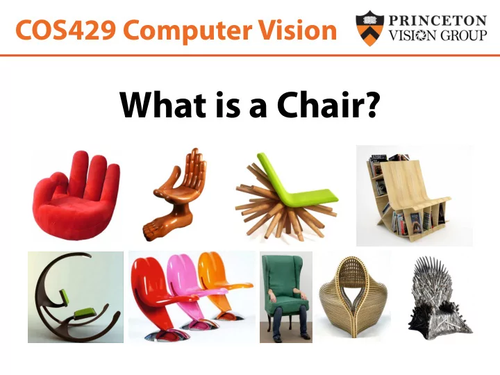
COS429 Computer Vision

What is a Chair?

The object

The object The texture

The object The texture The scene

Find a bottle:

Categories

Can’t do unless you do not care about few errors…

Instances Find these two toys

Can nail it

Instances vs. categories

Why do we care about recognition?

Perception of function: We can perceive the 3D shape, texture, material properties, without knowing about objects. But, the concept of category encapsulates also information about what can we do with those objects.

“We therefore include the perception of function as a proper –indeed, crucial- subject for vision science”, from Vision Science, chapter 9, Palmer.

The perception of function

• Direct perception (affordances): Gibson

Flat surface Horizontal Knee-high … Sittable upon Chair Chair Chair? Flat surface Horizontal Knee-high … Sittable upon Chair

• Mediated perception (Categorization)

Direct perception

Some aspects of an object function can be perceived directly

• Functional form: Some forms clearly

indicate to a function (“sittable-upon”, container, cutting device, …)

Sittable-upon Sittable-upon Sittable-upon It does not seem easy to sit-upon this…

Direct perception

Some aspects of an object function can be perceived directly

• Observer relativity: Function is observer

dependent

From http://lastchancerescueflint.org

Limitations of Direct Perception

The functions are the same at some level of description: we can put things inside in both and somebody will come later to empty them. However, we are not expected to put inside the same kinds of things…

Objects of similar structure might have very different functions

Not all functions seem to be available from direct visual information only.

Limitations of Direct Perception

Propulsion system Strong protective surface Something that looks like a door Sure, I can travel to space on this object

Visual appearance might be a very weak cue to function

Object recognition Is it really so hard?

This is a chair Find the chair in this image Output of normalized correlation

Object recognition Is it really so hard?

My biggest concern while making this slide was: how do I justify 50 years of research, and this course, if this experiment did work? Find the chair in this image Pretty much garbage Simple template matching is not going to make it

Object recognition Is it really so hard?

Find the chair in this image A “popular method is that of template matching, by point to point correlation of a model pattern with the image pattern. These techniques are inadequate for three- dimensional scene analysis for many reasons, such as occlusion, changes in viewing angle, and articulation of parts.” Nivatia & Binford, 1977.

Why is object recognition a hard task?

Challenges 1: view point variation

Michelangelo 1475-1564

Slides: course object recognition ICCV 2005

Challenges 2: illumination

slide credit: S. Ullman

Challenges 3: occlusion

Magritte, 1957

Slides: course object recognition ICCV 2005

Challenges 4: scale

Slides: course object recognition ICCV 2005

Challenges 5: deformation

Xu, Beihong 1943

Slides: course object recognition ICCV 2005

Challenges 6: intra-class variation

Slides: course object recognition ICCV 2005

Brady, M. J., & Kersten, D. (2003). Bootstrapped learning of novel objects. J Vis, 3(6), 413-422

Challenges 7: background clutter

Which level of categorization is the right one?

Car is an object composed of: a few doors, four wheels (not all visible at all times), a roof, front lights, windshield If you are thinking in buying a car, you might want to be a bit more specific about your categorization.

?

Entry-level categories

(Jolicoeur, Gluck, Kosslyn 1984)

• Typical member of a basic-level category

are categorized at the expected level

• Atypical members tend to be classified at

a subordinate level.

A bird An ostrich

Creation of new categories

A new class can borrow information from similar categories

Yes, object recognition is hard…

(or at least it seems so for now…)

Object recognition Is it really so hard?

So, let’s make the problem simpler: Block world

Nice framework to develop fancy math, but too far from reality…

Object Recognition in the Geometric Era: a Retrospective. Joseph L. Mundy. 2006

Object Recognition in the Geometric Era: a Retrospective. Joseph L. Mundy. 2006

Binford and generalized cylinders

Binford and generalized cylinders

Recognition by components

Irving Biederman Recognition-by-Components: A Theory of Human Image Understanding. Psychological Review, 1987.

Recognition by components

The fundamental assumption of the proposed theory, recognition-by-components (RBC), is that a modest set

• f generalized-cone components, called geons (N = 36),

can be derived from contrasts of five readily detectable properties of edges in a two-dimensional image: curvature, collinearity, symmetry, parallelism, and cotermination. The “contribution lies in its proposal for a particular vocabulary of components derived from perceptual mechanisms and its account of how an arrangement of these components can access a representation of an

• bject in memory.”

1) We know that this object is nothing we know 2) We can split this objects into parts that everybody will agree 3) We can see how it resembles something familiar: “a hot dog cart” “The naive realism that emerges in descriptions of nonsense objects may be reflecting the workings of a representational system by which objects are identified.”

A do-it-yourself example

Hypothesis

• Hypothesis: there is a small number of geometric

components that constitute the primitive elements of the

• bject recognition system (like letters to form words).
• “The particular properties of edges that are postulated to

be relevant to the generation of the volumetric primitives have the desirable properties that they are invariant over changes in orientation and can be determined from just a few points on each edge.”

• Limitation: “The modeling has been limited to concrete

entities with specified boundaries.” (count nouns) – this limitation is shared by many modern object detection algorithms.

Constraints on possible models of recognition

1) Access to the mental representation of an

• bject should not be dependent on absolute

judgments of quantitative detail 2) The information that is the basis of recognition should be relatively invariant with respect to

• rientation and modest degradation.

3) Partial matches should be computable. A theory

• f object interpretation should have some

principled means for computing a match for

• ccluded, partial, or new exemplars of a given

category.

Stages of processing

“Parsing is performed, primarily at concave regions, simultaneously with a detection of nonaccidental properties.”

Non accidental properties

Certain properties of edges in a two-dimensional image are taken by the visual system as strong evidence that the edges in the three-dimensional world contain those same properties. Non accidental properties, (Witkin & Tenenbaum,1983): Rarely be produced by accidental alignments of viewpoint and object features and consequently are generally unaffected by slight variations in viewpoint. ?

image

Examples:

• Colinearity
• Smoothness
• Symmetry
• Parallelism
• Cotermination

The high speed and accuracy of determining a given nonaccidental relation {e.g., whether some pattern is symmetrical) should be contrasted with performance in making absolute quantitative judgments of variations in a single physical attribute, such as length of a segment or degree of tilt or curvature. Object recognition is performed by humans in around 100ms.

“If contours are deleted at a vertex they can be restored, as long as there is no accidental filling-in. The greater disruption from vertex deletion is expected on the basis

• f their importance as diagnostic image features for the components.”

Recoverable Unrecoverable

From generalized cylinders to GEONS

“From variation over only two or three levels in the nonaccidental relations of four attributes of generalized cylinders, a set of 36 GEONS can be generated.” Geons represent a restricted form of generalized cylinders.

More GEONS

Objects and their geons

Scenes and geons

Mezzanotte & Biederman

Supercuadrics

Introduced in computer vision by A. Pentland, 1986.

What is missing?

The notion of geometric structure. Although they were aware of it, the previous works put more emphasis on defining the primitive elements than modeling their geometric relationships.

The importance of spatial arrangement

Parts and Structure approaches

With a different perspective, these models focused more on the geometry than on defining the constituent elements:

• Fischler & Elschlager 1973
• Yuille ‘91
• Brunelli & Poggio ‘93
• Lades, v.d. Malsburg et al. ‘93
• Cootes, Lanitis, Taylor et al. ‘95
• Amit & Geman ‘95, ‘99
• Perona et al. ‘95, ‘96, ’98, ’00, ’03, ‘04, ‘05
• Felzenszwalb & Huttenlocher ’00, ’04
• Crandall & Huttenlocher ’05, ’06
• Leibe & Schiele ’03, ’04
• Many papers since 2000

Figure from [Fischler & Elschlager 73]

Representation

• Object as set of parts

– Generative representation

• Model:

– Relative locations between parts – Appearance of part

• Issues:

– How to model location – How to represent appearance – Sparse or dense (pixels or regions) – How to handle occlusion/clutter

We will discuss these models more in depth later

But, despite promising initial results…things did not work out so well (lack of data, processing power, lack of reliable methods for low-level and mid- level vision) Instead, a different way of thinking about object detection started making some progress: learning based approaches and classifiers, which ignored low and mid-level vision. Maybe the time is here to come back to some of the earlier models, more grounded in intuitions about visual perception.

Neocognitron

Fukushima (1980). Hierarchical multilayered neural network S-cells work as feature-extracting cells. They resemble simple cells of the primary visual cortex in their response. C-cells, which resembles complex cells in the visual cortex, are inserted in the network to allow for positional errors in the features of the stimulus. The input connections of C-cells, which come from S-cells of the preceding layer, are fixed and invariable. Each C-cell receives excitatory input connections from a group

• f S-cells that extract the same feature, but from slightly different positions. The

C-cell responds if at least one of these S-cells yield an output.

Neocognitron

Learning is done greedily for each layer

Convolutional Neural Network

The output neurons share all the intermediate levels Le Cun et al, 98

Face detection and the success

• f learning based approaches
• The representation and matching of pictorial structures Fischler, Elschlager (1973).
• Face recognition using eigenfaces M. Turk and A. Pentland (1991).
• Human Face Detection in Visual Scenes - Rowley, Baluja, Kanade (1995)
• Graded Learning for Object Detection - Fleuret, Geman (1999)
• Robust Real-time Object Detection - Viola, Jones (2001)
• Feature Reduction and Hierarchy of Classifiers for Fast Object Detection in Video Images - Heisele, Serre,

Mukherjee, Poggio (2001)

• ….

Distribution-Based Face Detector

• Learn face and nonface models from examples [Sung and

Poggio 95]

• Cluster and project the examples to a lower dimensional space

using Gaussian distributions and PCA

• Detect faces using distance metric to face and nonface clusters

Distribution-Based Face Detector

• Learn face and nonface models from examples [Sung and

Poggio 95]

Training Database 1000+ Real, 3000+ VIRTUAL 50,0000+ Non-Face Pattern

Neural Network-Based Face Detector

• Train a set of multilayer perceptrons and

arbitrate a decision among all outputs [Rowley et al. 98]

Faces everywhere

59 http://www.marcofolio.net/imagedump/faces_everywhere_15_images_8_illusions.html

Paul Viola Michael J. Jones Mitsubishi Electric Research Laboratories (MERL) Cambridge, MA

Most of this work was done at Compaq CRL before the authors moved to MERL

Rapid Object Detection Using a Boosted Cascade of Simple Features

http://citeseer.ist.psu.edu/cache/papers/cs/23183/http:zSzzSzwww.ai.mit.eduzSzpeoplezSzviolazSzresearchzSzpublicationszSzICCV01-Viola-Jones.pdf/viola01robust.pdf

Manuscript available on web:

Face detection

Families of recognition algorithms

Bag of words models Voting models Constellation models Rigid template models

Sirovich and Kirby 1987 Turk, Pentland, 1991 Dalal & Triggs, 2006 Fischler and Elschlager, 1973 Burl, Leung, and Perona, 1995 Weber, Welling, and Perona, 2000 Fergus, Perona, & Zisserman, CVPR 2003 Viola and Jones, ICCV 2001 Heisele, Poggio, et. al., NIPS 01 Schneiderman, Kanade 2004 Vidal-Naquet, Ullman 2003

Shape matching Deformable models

Csurka, Dance, Fan, Willamowski, and Bray 2004 Sivic, Russell, Freeman, Zisserman, ICCV 2005 Berg, Berg, Malik, 2005 Cootes, Edwards, Taylor, 2001

(The lousy painter)

Discriminative vs. generative

10 20 30 40 50 60 70 0.05 0.1

x = data

• Generative model

10 20 30 40 50 60 70 0.5 1

x = data

• Discriminative model

10 20 30 40 50 60 70 80

• 1

1

x = data

• Classification function

(The artist)

Discriminative methods

Object detection and recognition is formulated as a classification problem.

Bag of image patches

Decision boundary

… and a decision is taken at each window about if it contains a target object or not.

Computer screen Background

In some feature space

Where are the screens?

The image is partitioned into a set of overlapping windows

Discriminative methods

106 examples

Nearest neighbor Shakhnarovich, Viola, Darrell 2003 Berg, Berg, Malik 2005 … Neural networks LeCun, Bottou, Bengio, Haffner 1998 Rowley, Baluja, Kanade 1998 … Support Vector Machines and Kernels Conditional Random Fields McCallum, Freitag, Pereira 2000 Kumar, Hebert 2003 … Guyon, Vapnik Heisele, Serre, Poggio, 2001 …

• Formulation: binary classification

Formulation

+1

• 1

x1 x2 x3 xN

… …

xN+1 xN+2 xN+M

• 1
• 1

? ? ? …

Training data: each image patch is labeled as containing the object or background Test data Features x = Labels y = Where belongs to some family of functions

• Classification function
• Minimize misclassification error

(Not that simple: we need some guarantees that there will be generalization)

Object representations

Explicit 3D models: use volumetric

• representation. Have an explicit model of

the 3D geometry of the object.

Appealing but hard to get it to work…

Object representations

Implicit 3D models: matching the input 2D view to view-specific representations.

Not very appealing but somewhat easy to get it to work…

Class experiment

Class ¡experiment ¡

Experiment ¡1: ¡draw ¡a ¡horse ¡(the ¡en3re ¡body, ¡ not ¡just ¡the ¡head) ¡in ¡a ¡white ¡piece ¡of ¡paper. ¡ ¡ ¡ Do ¡not ¡look ¡at ¡your ¡neighbor! ¡You ¡already ¡know ¡ how ¡a ¡horse ¡looks ¡like… ¡no ¡need ¡to ¡cheat. ¡

Class ¡experiment ¡

Experiment ¡2: ¡draw ¡a ¡horse ¡(the ¡en3re ¡body, ¡ not ¡just ¡the ¡head) ¡but ¡this ¡3me ¡chose ¡a ¡ viewpoint ¡as ¡weird ¡as ¡possible. ¡ ¡

3D object categorization

Despite we can categorize all three pictures as being views of a horse, the three pictures do not look as being equally typical views of

• horses. And they do not seem to be

recognizable with the same easiness.

Canonical Perspective

From Vision Science, Palmer

Examples of canonical perspective: In a recognition task, reaction time correlated with the ratings. Canonical views are recognized faster at the entry level. Experiment (Palmer, Rosch & Chase 81): participants are shown views of an object and are asked to rate “how much each one looked like the objects they depict” (scale; 1=very much like, 7=very unlike)

Canonical Viewpoint

Clocks are preferred as purely frontal

Histograms ¡of ¡oriented ¡gradients ¡for ¡ human ¡detec8on ¡ ¡

[Navneet ¡Dalal ¡and ¡Bill ¡Triggs, ¡2005] ¡

CVPR 2005

• 1. ¡Map ¡image ¡to ¡feature ¡Space ¡(HOG)

Human ¡detec3on ¡with ¡HOG: ¡Basic ¡Steps

• 1. ¡Map ¡image ¡to ¡feature ¡Space ¡(HOG) ¡

¡2. ¡Training ¡with ¡posi3ve ¡and ¡nega3ve ¡(linear ¡SVM) posi3ve ¡training ¡examples ¡ nega3ve ¡training ¡examples ¡

Human ¡detec8on ¡with ¡HOG: ¡Basic ¡Steps

• 1. ¡Map ¡image ¡to ¡feature ¡Space ¡(HOG) ¡

¡2. ¡Training ¡with ¡posi3ve ¡and ¡nega3ve ¡(linear ¡SVM) ¡

• 3. ¡Tes3ng ¡: ¡scan ¡image ¡in ¡all ¡scale ¡and ¡all ¡loca3on ¡

¡Binary ¡classifica3on ¡on ¡each ¡loca3on ¡

Human ¡detec8on ¡with ¡HOG: ¡Basic ¡Steps

Image ¡pyramid ¡

Problem ¡: ¡ Bounding ¡box ¡size ¡is ¡different ¡for ¡the ¡same ¡ ¡

• bject ¡(different ¡depth) ¡

¡ Solu3on ¡1: ¡ Resize ¡the ¡box ¡and ¡do ¡mul3ple ¡convolu3on? ¡ Not ¡ideal ¡: ¡ It ¡will ¡change ¡the ¡feature ¡dimension, need ¡ to ¡retrain ¡the ¡SVM ¡for ¡each ¡scale. ¡

Image ¡pyramid ¡

Solu3on ¡2: ¡ Resize ¡the ¡image ¡and ¡do ¡mul3ple ¡convolu3on?-> ¡image ¡pyramid ¡ Image ¡is ¡smaller ¡~ ¡box ¡is ¡bigger ¡ Image ¡is ¡larger ¡~ ¡box ¡is ¡smaller ¡

• 1. ¡Map ¡image ¡to ¡feature ¡Space ¡(HOG) ¡

¡2. ¡Training ¡with ¡posi3ve ¡and ¡nega3ve ¡(linear ¡SVM) ¡

• 3. ¡Tes3ng ¡: ¡scan ¡image ¡in ¡all ¡scale ¡and ¡all ¡loca3on ¡

¡Binary ¡classifica3on ¡on ¡each ¡loca3on ¡

Human ¡detec8on ¡with ¡HOG: ¡Basic ¡Steps

• 1. ¡Map ¡image ¡to ¡feature ¡Space ¡(HOG) ¡

¡2. ¡Training ¡with ¡posi3ve ¡and ¡nega3ve ¡(linear ¡SVM) ¡

• 3. ¡Tes3ng ¡: ¡scan ¡image ¡in ¡all ¡scale ¡and ¡all ¡loca3on ¡
• 4. ¡Report ¡box： ¡non-­‑maximum ¡suppression ¡ ¡

Human ¡detec8on ¡with ¡HOG: ¡Basic ¡Steps

Final ¡Boxes ¡ Detector ¡response ¡map ¡ A]er ¡thresholding ¡ ¡ A]er ¡non-­‑maximum ¡suppression ¡

Training: ¡ ¡Train ¡a ¡classifier ¡describe ¡the ¡detec3on ¡ target ¡ ¡ ¡ ¡ Tes3ng ¡: ¡ Detec3on ¡by ¡binary ¡classifica3on ¡on ¡all ¡ loca3on ¡ Summary ¡of ¡Basic ¡object ¡detec8on ¡Steps

HOG ¡descriptor ¡

HOG: Gradients ¡

• Compress ¡image ¡to ¡64x128 ¡pixels ¡
• Convolu3on ¡with ¡[-­‑1 ¡0 ¡1] ¡[-­‑1;0; ¡1] ¡filters ¡
• Compute ¡gradient ¡magnitude ¡+ ¡direc3on ¡ ¡
• For ¡each ¡pixel: take ¡the ¡color ¡channel ¡with ¡

greatest ¡magnitude ¡ ¡as ¡final ¡gradient ¡ ¡

HOG: ¡Cell ¡histograms ¡

• Divide ¡the ¡image ¡to ¡cells, each ¡cell ¡8x8 ¡pixels ¡ ¡
• Snap ¡each ¡pixel’s ¡direc3on ¡to ¡one ¡of ¡18 ¡

gradient ¡ ¡orienta3ons ¡ ¡

• Build ¡histogram ¡pre-­‑cell ¡using ¡magnitudes ¡ ¡

Histogram ¡interpola8on ¡example ¡

• Interpolated trilinearly:

– Bilinearly into spatial cells – Linearly into orientation bins

Normaliza8on ¡

Cell ¡ Cell ¡ Current ¡cell ¡: ¡1x18 ¡histogram ¡ ¡ Block: ¡2x2 ¡cell ¡ ¡overlapping ¡with ¡current ¡cell ¡

• 1. contrast ¡sensi8ve ¡features: ¡18 ¡orienta3on ¡-­‑> ¡18 ¡dim ¡
• 2. contrast ¡insensi8ve ¡features: ¡9 ¡orienta3on ¡-­‑> ¡9 ¡dim ¡

Normalize ¡4 ¡3mes ¡by ¡its ¡neighbor ¡blocks, ¡and ¡average ¡them ¡ ¡ ¡

• 3. ¡texture ¡features: ¡sum ¡of ¡the ¡magnitude ¡over ¡all ¡orienta3on ¡and ¡normalize ¡4 ¡

3me,not ¡average ¡-­‑> ¡4 ¡dim ¡ ¡ ¡ In ¡total ¡each ¡cell ¡: ¡18+9+4 ¡dimension ¡of ¡feature ¡ ¡

Final ¡Descriptor ¡

• Concatena3on ¡the ¡normalized ¡histogram ¡

¡ Visualiza3on: ¡

HOG ¡Descriptor: ¡

1. Compute ¡gradients ¡on ¡an ¡image ¡ region ¡of ¡64x128 ¡pixels ¡ 2. Compute ¡histograms ¡on ¡‘cells’ ¡of ¡ typically ¡8x8 ¡pixels ¡(i.e. ¡8x16 ¡cells) ¡ ¡ 3. Normalize ¡histograms ¡within ¡

• verlapping ¡blocks ¡of ¡cells ¡

¡ 4. Concatenate ¡histograms ¡ It ¡is ¡a ¡typical ¡procedure ¡of ¡ ¡feature ¡extrac8on ¡! ¡ ¡

Feature ¡Engineering ¡

• Developing ¡a ¡feature ¡descriptor ¡requires ¡a ¡

lot ¡of ¡engineering ¡

– Tes3ng ¡of ¡parameters ¡(e.g. ¡size ¡of ¡cells, ¡blocks, ¡ number ¡of ¡cells ¡in ¡a ¡block, ¡size ¡of ¡overlap) ¡ – Normaliza3on ¡schemes ¡ ¡

• An ¡extensive ¡evalua3on ¡was ¡performed ¡to ¡

make ¡these ¡design ¡desicca3ons ¡

• It’s ¡not ¡only ¡the ¡idea, ¡but ¡also ¡the ¡

engineering ¡effort ¡

Problem ¡? ¡

Single, ¡rigid ¡template ¡usually ¡not ¡enough ¡to ¡ represent ¡a ¡category. ¡

• Many ¡object ¡categories ¡look ¡very ¡different ¡from ¡

different ¡viewpoints, ¡or ¡style ¡ ¡ ¡ ¡

• Many ¡objects ¡(e.g. ¡humans) ¡are ¡ar3culated, ¡or ¡

have ¡parts ¡that ¡can ¡vary ¡in ¡configura3on ¡ ¡

¡

Solu8on ¡: ¡

• Exemplar ¡SVM: ¡Ensemble ¡of ¡Exemplar-­‑SVMs ¡

for ¡Object ¡Detec3on ¡and ¡Beyond ¡

• Part ¡Based ¡Model ¡

Exemplar-SVM

• S3ll ¡a ¡rigid ¡template,but ¡train ¡a ¡separate ¡SVM ¡

for ¡each ¡posi3ve ¡instance ¡

For ¡each ¡category ¡it ¡can ¡has ¡exemplar ¡with ¡different ¡size ¡aspect ¡ra3o ¡

• Handel ¡the ¡intra-­‑category ¡variance ¡naturally,

without ¡using ¡complicated ¡model. ¡

• Compare ¡to ¡nearest ¡neighbor ¡approach:

make ¡use ¡of ¡nega3ve ¡data ¡and ¡train ¡a ¡ discrimina3ve ¡object ¡detector ¡

• Explicit ¡correspondence ¡from ¡detec3on ¡result ¡

to ¡training ¡exemplar ¡ ¡

Benefit ¡from ¡Exemplar-SVM ¡?

• Explicit ¡correspondence ¡from ¡detec3on ¡result ¡

to ¡training ¡exemplar ¡ ¡

Benefit ¡from ¡Exemplar-SVM ¡?

We ¡not ¡only ¡know ¡it ¡is ¡train,but ¡also ¡its ¡orienta3on ¡ and ¡type! ¡

Benefit ¡from ¡Exemplar-SVM ¡?

We ¡can ¡do ¡even ¡more ¡ ¡

Training ¡Exemplar-SVM ¡

Objec3ve ¡Func3on: ¡ ¡ Learn ¡the ¡w ¡that ¡minimize ¡the ¡ ¡objec3ve ¡ func3on, equivalent ¡to ¡maximize ¡the ¡margin ¡ ¡ ¡ ¡ ¡

• ­‑1 ¡

h(x) ¡=0 ¡

• ­‑1 ¡

Hard ¡Nega3ve ¡Mining ¡

Windows ¡from ¡images ¡not ¡containing ¡any ¡in-­‑ class ¡instances: ¡but ¡there ¡is ¡too ¡many! ¡ 2,000 ¡images ¡x ¡10,000 ¡windows ¡per ¡image ¡= ¡ 20M ¡nega3ves ¡ ¡ ¡ Find ¡ones ¡that ¡you ¡get ¡wrong ¡by ¡a ¡search, ¡and ¡train ¡

• n ¡these ¡hard ¡ones ¡

Hard ¡Nega3ve ¡Mining ¡

While ¡: ¡ i ¡!= ¡m ¡or ¡Nhard ¡not ¡empty ¡ ¡for ¡i= ¡1to ¡n ¡do ¡ ¡ ¡ D ¡= ¡detect(b,w,Ji) ¡ ¡ ¡ ¡ Ni= ¡D.conf ¡> ¡threshold ¡& ¡D ¡not ¡overlap ¡with ¡Bi ¡

¡ ¡ ¡ ¡ ¡ Add ¡Ni ¡to ¡Nhard ¡

¡ ¡ ¡ ¡if ¡|Nhard| ¡> ¡memory-limit, ¡then ¡break; ¡

¡end ¡

¡[SVnew,bnew,wnew]=trainSVM(E, ¡[Nrandom,SV]) ¡ ¡SV ¡= ¡[SV; ¡SVnew] ¡ end ¡ Input ¡: ¡Posi3ve ¡: ¡exemplar ¡E ¡ ¡ ¡ ¡Nega3ve ¡: ¡images ¡and ¡bounding ¡boxes ¡for ¡this ¡category ¡ ¡ ¡ ¡ N={(J1,B1), ¡(J2,B2),…(Jm,Bm)} ¡ Ini)alize: random ¡pick ¡m ¡patches ¡Nrandom ¡from ¡N ¡that ¡not ¡overlap ¡with ¡ ¡ ¡ ¡ ¡[SV,b,w]=trainSVM(E, ¡Nrandom) ¡ Hard ¡nega)ve ¡mining ¡ ¡ ¡

Embarrassingly ¡Parallel ¡

Objects ¡are ¡represented ¡by ¡features ¡of ¡parts ¡and ¡ spa3al ¡rela3ons ¡between ¡parts ¡

Part ¡Based ¡detector ¡ ¡

• How ¡to ¡defined ¡the ¡parts ¡for ¡one ¡object ¡

category ¡ ¡

• How ¡to ¡represent ¡their ¡spa3al ¡rela3on ¡shape ¡ ¡
• How ¡to ¡combine ¡parts ¡detec3on ¡and ¡spa3al ¡

rela3ons ¡to ¡obtained ¡the ¡final ¡detec3on ¡

Part ¡Based ¡detector ¡ ¡

Structure ¡models ¡

Voting models Constellation models Deformable models

• Many parts (>100)
• Few parts (~6)
• No parts

From wikipedia: Perhaps the most famous part of the work is chapter XVII, "The Comparison of Related Forms," where Thompson explored the degree to which differences in the forms of related animals could be described by means of relatively simple mathematical transformations.

Structure ¡models ¡

Voting models Constellation models Deformable models

• Many parts (>100)
• Few parts (~6)
• No parts

B a g

• f

w

• r

d s

• N
• s

t r u c t u r e !

Object Bag of ‘words’

Slide credit: Fei fei

Analogy ¡to ¡documents ¡

Of all the sensory impressions proceeding to the brain, the visual experiences are the dominant ones. Our perception of the world around us is based essentially on the messages that reach the brain from our eyes. For a long time it was thought that the retinal image was transmitted point by point to visual centers in the brain; the cerebral cortex was a movie screen, so to speak, upon which the image in the eye was projected. Through the discoveries of Hubel and Wiesel we now know that behind the origin of the visual perception in the brain there is a considerably more complicated course of events. By following the visual impulses along their path to the various cell layers of the optical cortex, Hubel and Wiesel have been able to demonstrate that the message about the image falling on the retina undergoes a step- wise analysis in a system of nerve cells stored in columns. In this system each cell has its specific function and is responsible for a specific detail in the pattern of the retinal image.

sensory, brain, visual, perception, retinal, cerebral cortex, eye, cell, optical nerve, image Hubel, Wiesel

China is forecasting a trade surplus of $90bn (£51bn) to $100bn this year, a threefold increase on 2004's $32bn. The Commerce Ministry said the surplus would be created by a predicted 30% jump in exports to $750bn, compared with a 18% rise in imports to $660bn. The figures are likely to further annoy the US, which has long argued that China's exports are unfairly helped by a deliberately undervalued yuan. Beijing agrees the surplus is too high, but says the yuan is only one factor. Bank of China governor Zhou Xiaochuan said the country also needed to do more to boost domestic demand so more goods stayed within the

• country. China increased the value of the

yuan against the dollar by 2.1% in July and permitted it to trade within a narrow band, but the US wants the yuan to be allowed to trade

• freely. However, Beijing has made it clear that

it will take its time and tread carefully before allowing the yuan to rise further in value.

China, trade, surplus, commerce, exports, imports, US, yuan, bank, domestic, foreign, increase, trade, value

Slide credit: Fei fei

• P. ¡Felzenszwalb, ¡R. ¡Girshick, ¡D. ¡McAllester, ¡D. ¡Ramanan, ¡

Object ¡Detec3on ¡with ¡Discrimina3vely ¡Trained ¡Part ¡Based ¡Models, ¡PAMI ¡32(9), ¡ 2010 ¡

DPM ¡: ¡Object ¡Detec8on ¡with ¡ Discrimina8vely ¡Trained ¡Part ¡Based ¡Models ¡

DPM: ¡overview ¡

• ¡Each ¡category ¡detector ¡has ¡mixture ¡of ¡

deformable ¡part ¡models ¡(components) ¡

• ¡Each ¡component ¡has ¡global ¡template ¡+ ¡

deformable ¡parts ¡

• ¡Fully ¡trained ¡from ¡bounding ¡boxes ¡alone ¡

(Latent ¡SVM) ¡

DPM: ¡component ¡ ¡

• Each ¡category ¡detector ¡has ¡mixture ¡of ¡

component ¡ ¡for ¡different ¡aspect ¡ra3o ¡(handle ¡ intra-­‑class ¡variance) ¡

• Each ¡component ¡has ¡a ¡it’s ¡own ¡DPM ¡model ¡

Deformable part models

Model encodes local appearance + pairwise geometry

Source: Deva Ramanan

DPM: ¡component ¡ ¡

Example models

Source: Deva Ramanan

Example models

Source: Deva Ramanan

Example models

PASCAL Visual Object Challenge

5000 training images 5000 testing images 20 everyday object categories

aeroplane bike bird boat bottle bus car cat chair cow table dog horse motorbike person plant sheep sofa train tv

Source: Deva Ramanan

5 years of PASCAL people detection

average precision

Discriminative mixtures of star models 2007-2010 Felzenszwalb,

McAllester, Ramanan CVPR 2008 Felzenszwalb, Girshick, McAllester, and Ramanan PAMI 2009

1% to 45% in 5 years

Source: Deva Ramanan

Evaluation: Precision & Recall

Precision = TP / (TP + FP) Recall = TP / (TP + FN)

Object No Object Truth Object No Object Algorithm Prediction

True Positive True Negative False Positive False Negative

Truth Prediction

Intersection Over Union =

/

Evaluation: Precision & Recall

Table

Concept Review

• Object vs. Scene vs. Texture
• Instances vs. categories
• Mediated vs. Directed
• Entry-level vs. Fine-grained
• Knowledge-based vs. Data-driven
• Explicit 3D vs. Implicit 3D (view-based)
• Whole vs. parts
• Discriminative vs. generative
• Structure vs. Bag-of-Words