1-Bucket-Theta: Map 1-Bucket-Theta: Reduce Col T 1 6 Row - - PDF document

1 bucket theta map 1 bucket theta reduce
SMART_READER_LITE
LIVE PREVIEW

1-Bucket-Theta: Map 1-Bucket-Theta: Reduce Col T 1 6 Row - - PDF document

10/20/2011 1-Bucket-Theta: Map 1-Bucket-Theta: Reduce Col T 1 6 Row Input: tuple x S T, Input: ( ID, [(x 1 , origin 1 ),..., (x k , origin k )] ) 1 S1.A=5 S2.A=7 matrix-to-reducer mapping lookup table 1 2 S3.A=7 S4.A=8


slide-1
SLIDE 1

10/20/2011 1

1-Bucket-Theta: Map

  • Input: tuple xST,

matrix-to-reducer mapping lookup table

  • 1. If xS then
  • 1. matrixRow = random( 1, |S| )
  • 2. Forall regionID in lookup.getRegions( matrixRow )

1. Output ( regionID, (x, “S”) )

  • 2. Else
  • 1. matrixCol = random( 1, |T| )
  • 2. Forall regionID in lookup.getRegions( matrixCol )

1. Output ( regionID, (x, “T”) )

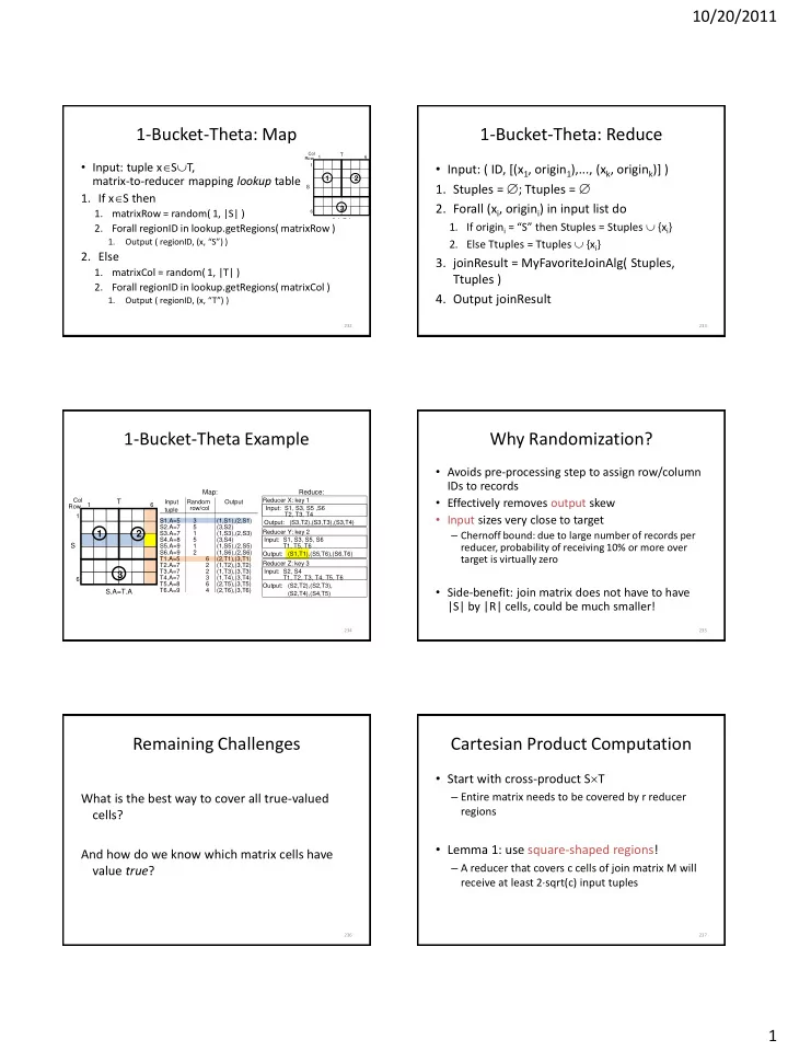
232 T6.A=9 T5.A=8 T4.A=7 T2.A=7 T1.A=5 S6.A=9 S5.A=9 S4.A=8 S3.A=7 S2.A=7 S1.A=5 T3.A=7

1 2 3

Row Col S T S.A=T.A 1 6 1 6

1-Bucket-Theta: Reduce

  • Input: ( ID, [(x1, origin1),..., (xk, origink)] )
  • 1. Stuples = ; Ttuples = 
  • 2. Forall (xi, origini) in input list do
  • 1. If origini = “S” then Stuples = Stuples  {xi}
  • 2. Else Ttuples = Ttuples  {xi}
  • 3. joinResult = MyFavoriteJoinAlg( Stuples,

Ttuples )

  • 4. Output joinResult

233

1-Bucket-Theta Example

234

Reduce: 5 1 2 1 5 6 2 2 3 6 4 Random row/col (2,T6),(3,T6) (2,T5),(3,T5) (1,T4),(3,T4) (1,T3),(3,T3) (1,T2),(3,T2) (2,T1),(3,T1) (1,S6),(2,S6) (1,S5),(2,S5) (3,S4) (1,S3),(2,S3) (3,S2) (1,S1),(2,S1) T6.A=9 T5.A=8 T4.A=7 T2.A=7 T1.A=5 S6.A=9 S5.A=9 S4.A=8 S3.A=7 S2.A=7 S1.A=5 T3.A=7 Input tuple Output

1 2 3

Reducer X: key 1 Input: S1, S3, S5 ,S6 T2, T3, T4 (S3,T2),(S3,T3),(S3,T4) Output: Reducer Y: key 2 Input: Output: S1, S3, S5, S6 T1, T5, T6 (S1,T1),(S5,T6),(S6,T6) Reducer Z: key 3 Input: S2, S4 T1, T2, T3, T4, T5, T6 (S2,T4),(S4,T5) (S2,T2),(S2,T3), Output: Map: Row Col

S T S.A=T.A

1 6 1 6 3

Why Randomization?

  • Avoids pre-processing step to assign row/column

IDs to records

  • Effectively removes output skew
  • Input sizes very close to target

– Chernoff bound: due to large number of records per reducer, probability of receiving 10% or more over target is virtually zero

  • Side-benefit: join matrix does not have to have

|S| by |R| cells, could be much smaller!

235

Remaining Challenges

What is the best way to cover all true-valued cells? And how do we know which matrix cells have value true?

236

Cartesian Product Computation

  • Start with cross-product ST

– Entire matrix needs to be covered by r reducer regions

  • Lemma 1: use square-shaped regions!

– A reducer that covers c cells of join matrix M will receive at least 2sqrt(c) input tuples

237

slide-2
SLIDE 2

10/20/2011 2

Optimal Cover for M

  • Need to cover all |S||T| matrix cells

– Lower bound for max-reducer-output: |S||T|/r – Lemma 1 implies lower bound for max-reducer- input: 2sqrt(|S||T|/r)

  • Can we match these lower bounds?

– YES: Use r squares, each sqrt(|S||T|/r) cells wide/tall

  • Can this be achieved for given S, T, r?

238

Easy Case

  • |S|, |T| are both multiples of sqrt(|S||T|/r)
  • Optimal!

239

Optimal square region S T Join matrix (cross-product)

Also Easy

  • |S| < |T|/r

– Implies |S| < sqrt(|S||T|/r) – Lower bound for input not achievable

  • Optimal: use rectangles of size |S| by |T|/r

240

“Idealistic” square region S T Actual optimal region S T

Hard Case

  • |T|/r  |S|  |T| and at least one is not

multiple of sqrt(|S||T|/r)

241

Optimal square region S T 9 regions:

  • 6 fit
  • 3 do not fit

Solution For Hard Case

  • “Inflate” squares until they just cover the

matrix

– Worst case: only one square did fit initially, but leftover just too small to fit more rows or columns

242

Need to at most double side-length of optimal square

Near-Optimality For Cross-Product

  • Every region has less than 4sqrt(|S||T|/r) input

records

– Lower bound: 2sqrt(|S||T|/r)

  • Every region contains less than 4|S||T|/r cells

– Lower bound: |S||T|/r

  • Summary: max-reducer-input and max-reducer-
  • utput are within a factor of 2 and 4 of the lower

bound, respectively

– Usually much better: if 10 by 10 squares fit initially, they are within a factor of 1.1 and 1.21 of lower bound!

243

slide-3
SLIDE 3

10/20/2011 3

From Cross-Product To Joins

  • Near-optimality only shown for cross-product
  • Randomization of 1-Bucket-Theta tends to

distribute output very evenly over regions

– Join-specific mapping unlikely to improve max- reducer-output significantly – 1-Bucket-Theta wins for output-size dominated joins

  • Join-specific mapping has to beat 1-Bucket-Theta
  • n input cost!

– Avoid covering empty matrix regions

244

Finding Empty Matrix Regions

  • For a given matrix region, prove that it

contains no join result

  • Need statistics about S and T
  • Need simple enough join predicate

– Histogram bucket: S.A > 8  T.A < 7 – Join predicate: S.A = T.A – Easy to show that bucket property implies negation of join predicate

  • Not possible for “blackbox” join predicates

245

Approximate Join Matrix

246

True join matrix Histogram boundaries Candidate cells to be covered by algorithm

What Can We Do?

  • Even if we could guess a better algorithm than

1-Bucket-Theta, we cannot use it unless we can prove that it does not miss any join results

  • Can do this for many popular join types

– Equi-join: S.A = T.A – Inequality-join: S.A  T.A – Band-join: R.A - 1  S.A  R.A + 2

  • Need histograms (easy and cheap to compute)

247

M-Bucket-I

  • Uses Multiple-bucket histograms to minimize

max-reducer-Input

  • First identifies candidate cells
  • Then tries to cover all candidate cells with r

regions

– Binary search over max-reducer-input values

  • Min: 2sqrt(#candidateCells / r); max: |S|+|T|

– Works on block of consecutive rows

  • Find “best” block (most candidate cells covered per region)
  • Continue with next block, until all candidate cells covered, or

running out of regions

248

M-Bucket-I Illustration

249

MaxInput = 3 Block: row 1 Score: 1 Block: rows 1-2 Score: 1.5 Best: And so on.

slide-4
SLIDE 4

10/20/2011 4

M-Bucket-O

  • Similar to M-Bucket-I, but tries to minimize

max-reducer-Output

  • Binary search over max-reducer-output values
  • Problem: estimate number of result cells in

regions inside a histogram bucket

– Estimate can be poor, even for fine-grained histogram – Input-size estimation much more accurate than

  • utput-size estimation

250

Extension: Memory-Awareness

  • Input for region might exceed reducer memory
  • Solutions

– Use I/O-based join implementation in Reduce, or – Create more (and hence smaller) regions

  • 1-Bucket-Theta: use squares of side-length

Mem/2

  • M-Bucket-I: Instead of binary search on max-

reducer-input, set it immediately to Mem

  • Similar for M-Bucket-O

251

Experiments: Basic Setup

  • 10-machine cluster

– Quad-core Xeon 2.4GHz, 8MB cache, 8GB RAM, two 250GB 7.2K RPM hard disks

  • Hadoop 0.20.2

– One machine head node, other nine worker nodes – One Map or Reduce task per core – DFS block size of 64MB – Data stored on all 10 machines

252

Data Sets

  • Cloud

– Cloud reports from ships and land stations – 382 million records, 28 attributes, 28.8GB total size

  • Cloud-5-1, Cloud-5-2

– Independent random samples from Cloud, each with 5 million records

  • Synth-

– Pair of data sets of 5 million records each – Record is single integer between 1 and 1000 – Data set 1: uniformly generated – Data set 2: Zipf distribution with parameter 

  • For =0, data is perfectly uniform

253

Skew Resistance: Equi-Join

  • 1-Bucket-Theta vs. standard equi-join algorithm
  • Output-size dominated join

– Max-reducer-output determines runtime

254

1-Bucket-Theta Standard algorithm Data Set Output size (billion) Output imbalance Runtime (secs) Output Imbalance Runtime (secs) Synth-0 25.00 1.0030 657 1.001 701 Synth-0.4 24.99 1.0023 650 1.254 722 Synth-0.6 24.98 1.0033 676 1.778 923 Synth-0.8 24.95 1.0068 678 3.010 1482 Synth-1 24.91 1.0089 667 5.312 2489

Selective Band-Join

SELECT S.date, S.longitude, S.latitude, T.latitude FROM Cloud AS S, Cloud AS T WHERE S.date = T.date AND S.longitude = T.longitude AND ABS(S.latitude - T.latitude) <= 10

  • 390M output vs. 764M input records
  • M-Bucket-I for different histogram granularities

255

slide-5
SLIDE 5

10/20/2011 5

M-Bucket-I Results

256

Runtime for MapReduce only! 10-run averages (stdev < 15%)

M-Bucket-I Details

  • M-Bucket-I for 1-bucket histogram is improved version
  • f original 1-Bucket-Theta

– 1-Bucket-Theta might keep reducers idle

  • Out-of-memory for 1-bucket and 100-bucket cases

– Used memory-aware version of algorithm – Creates cr regions for r reducers for smallest integer c that allows in-memory processing

  • Input duplication rate: total mapper output size vs.

total mapper input size

– 31.22, 8.92, 1.93, 1.043, 1.00048, 1.00025 for histograms with 1, 10, 100, 1000, 10K, 100k, and 1M buckets

257

Not-So-Selective Band-Join

SELECT S.latitude, T.latitude FROM Cloud-5-1 AS S, Cloud-5-2 AS T WHERE ABS(S.latitude-T.latitude) <= 2

  • 22 billion output vs. 10 million input records
  • M-Bucket-O for different histogram

granularities

258

M-Bucket-O Results

259

Runtime for MapReduce only! 10-run averages (stdev < 4%)

M-Bucket-O Details

  • M-Bucket-O for 1-bucket histogram is

improved version of original 1-Bucket-Theta

  • Data set has 5951 distinct latitude values
  • Input duplication rate: total mapper output

size vs. total mapper input size

– 7.50, 4.14, 1.46, 1.053, 1.035 for histograms with 1, 10, 100, 1000, and 5951 buckets

260 261

Step Number of histogram buckets 1 10 100 1000 10,000 100,000 1,000,000 Quantiles 115 120 117 122 124 122 Histogram 140 145 147 157 167 604 Heuristic 74 9 0.8 1.5 17 118 111 Join 49,384 10,905 1157 595 548 540 536 Total 49,458 11169 1423 861 844 949 1373 Step Number of histogram buckets 1 10 100 1000 5951 Quantiles 4.5 4.5 4.8 4.9 Histogram 26.2 25.8 25.6 25.6 Heuristic 0.04 0.04 0.05 0.24 0.81 Join 1279 2483 1597 1369 1188 Total 1279 2514 1627 1399 1219 M-Bucket-I on Cloud data set (input-size dominated join): M-Bucket-O on Cloud-5 data sets (output-size dominated join):

Detailed cost breakdown

slide-6
SLIDE 6

10/20/2011 6

Summary

  • Join model for creation and reasoning about

parallel algorithms

  • Near-optimal randomized algorithm for
  • utput-size dominated joins
  • Improved heuristics for popular very selective

joins

262

Future Directions

  • Explore broader model applicability

– Very general model – Works for size-skewed joins where one set fits in memory

  • Improves completion time of Map-only implementation

– Algorithm can be executed sequentially

  • Can tune it to available memory
  • Multi-way theta-joins
  • Optimizer to select best implementation for given

join problem

263