1 Tracking and Recursive estimation Recursive estimation - - PDF document

1

1

6.891

Computer Vision and Applications

• Prof. Trevor. Darrell

Lecture 16: Tracking

– Density propagation – Linear Dynamic models / Kalman filter – Data association – Multiple models

Readings: F&P Ch 17

2

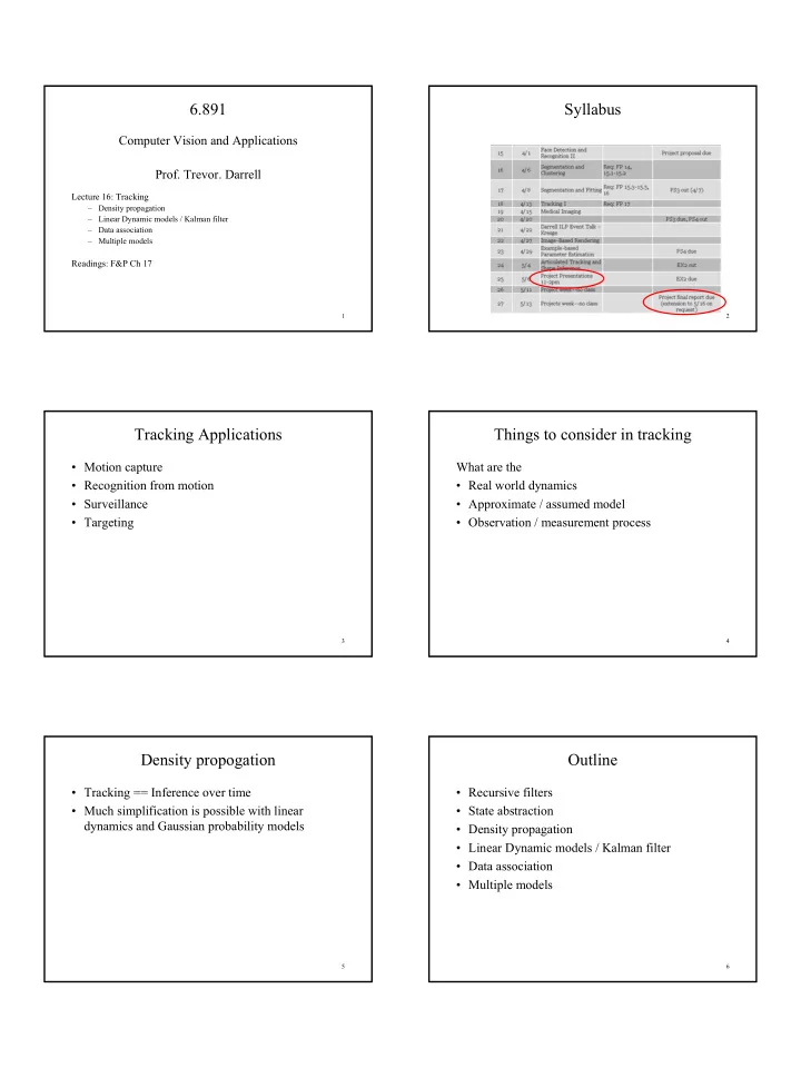
Syllabus

3

• Motion capture
• Recognition from motion
• Surveillance
• Targeting

Tracking Applications

4

What are the

• Real world dynamics
• Approximate / assumed model
• Observation / measurement process

Things to consider in tracking

5

• Tracking == Inference over time
• Much simplification is possible with linear

dynamics and Gaussian probability models

Density propogation

6

• Recursive filters
• State abstraction
• Density propagation
• Linear Dynamic models / Kalman filter
• Data association
• Multiple models

Outline

2

7

• Real-time / interactive imperative.
• Task: At each time point, re-compute estimate of

position or pose.

– At time n, fit model to data using time 0…n – At time n+1, fit model to data using time 0…n+1

• Repeat batch fit every time?

Tracking and Recursive estimation

8

• Decompose estimation problem

– part that depends on new observation – part that can be computed from previous history

• E.g., running average:

at = α at-1 + (1-α) yt

• Linear Gaussian models: Kalman Filter
• First, general framework…

Recursive estimation

9

Tracking

• Very general model:

– We assume there are moving objects, which have an underlying state X – There are measurements Y, some of which are functions of this state – There is a clock

• at each tick, the state changes
• at each tick, we get a new observation
• Examples

– object is ball, state is 3D position+velocity, measurements are stereo pairs – object is person, state is body configuration, measurements are frames, clock is in camera (30 fps)

10

Three main issues in tracking

11

Simplifying Assumptions

12

Tracking as induction

• Assume data association is done

– we’ll talk about this later; a dangerous assumption

• Do correction for the 0’th frame
• Assume we have corrected estimate for i’th frame

– show we can do prediction for i+1, correction for i+1

3

13

Base case

14

Induction step

given

15

Induction step

given

16

Linear dynamic models

• A linear dynamic model has the form
• This is much, much more general than it looks, and extremely

powerful yi = N Mixi;Σmi

( )

xi = N Di−1xi−1;Σdi

( )

17

Examples

• Drifting points

– assume that the new position of the point is the old one, plus noise D = Id yi = N Mixi;Σmi

( )

xi = N Di−1xi−1;Σdi

( )

cic.nist.gov/lipman/sciviz/images/random3.gif http://www.grunch.net/synergetics/images/random 3.jpg

18

Constant velocity

• We have

– (the Greek letters denote noise terms)

• Stack (u, v) into a single state vector

– which is the form we had above ui = ui−1 + ∆tvi−1 + εi vi = vi−1 + ςi u v      

i

= 1 ∆t 1       u v      

i−1

+ noise yi = N Mixi;Σmi

( )

xi = N Di−1xi−1;Σdi

( )

4

19

position position

Constant Velocity Model

velocity time measurement,position time

20

Constant acceleration

• We have

– (the Greek letters denote noise terms)

• Stack (u, v) into a single state vector

– which is the form we had above ui = ui−1 + ∆tvi−1 + εi vi = vi−1 + ∆tai−1 +ς i ai = ai−1 + ξi u v a        

i

= 1 ∆t 1 ∆t 1         u v a        

i−1

+ noise yi = N Mixi;Σmi

( )

xi = N Di−1xi−1;Σdi

( )

21

time position position velocity

Constant Acceleration Model

22

Assume we have a point, moving on a line with a periodic movement defined with a differential eq: can be defined as with state defined as stacked position and velocity u=(p, v)

Periodic motion

yi = N Mixi;Σmi

( )

xi = N Di−1xi−1;Σdi

( )

23

Take discrete approximation….(e.g., forward Euler integration with ∆t stepsize.)

Periodic motion

yi = N Mixi;Σmi

( )

xi = N Di−1xi−1;Σdi

( )

24

• Independence assumption
• Velocity and/or acceleration augmented position
• Constant velocity model equivalent to

– velocity == – acceleration == – could also use , etc.

Higher order models

5

25

The Kalman Filter

• Key ideas:

– Linear models interact uniquely well with Gaussian noise - make the prior Gaussian, everything else Gaussian and the calculations are easy – Gaussians are really easy to represent --- once you know the mean and covariance, you’re done

26

Recall the three main issues in tracking

(Ignore data association for now)

27

The Kalman Filter

[figure from http://www.cs.unc.edu/~welch/kalman/kalmanIntro.html]

28

The Kalman Filter in 1D

• Dynamic Model
• Notation

Predicted mean Corrected mean

29

The Kalman Filter

30

Prediction for 1D Kalman filter

• The new state is obtained by

– multiplying old state by known constant – adding zero-mean noise

• Therefore, predicted mean for new state is

– constant times mean for old state

• Old variance is normal random variable

– variance is multiplied by square of constant – and variance of noise is added.

6

31 32

The Kalman Filter

33

Correction for 1D Kalman filter

Notice:

– if measurement noise is small, we rely mainly on the measurement, – if it’s large, mainly on the prediction – σ does not depend on y

34 35

position position

Constant Velocity Model

velocity time

36

position and measurement time

7

37 38

The o-s give state, x-s measurement.

39

The o-s give state, x-s measurement.

40

Smoothing

• Idea

– We don’t have the best estimate of state - what about the future? – Run two filters, one moving forward, the other backward in time. – Now combine state estimates

• The crucial point here is that we can obtain a smoothed

estimate by viewing the backward filter’s prediction as yet another measurement for the forward filter

41 42

8

43 44

n-D

Generalization to n-D is straightforward but more complex.

45

n-D

Generalization to n-D is straightforward but more complex.

46

n-D Prediction

Generalization to n-D is straightforward but more complex. Prediction:

• Multiply estimate at prior time with forward model:
• Propagate covariance through model and add new noise:

47

n-D Correction

Generalization to n-D is straightforward but more complex. Correction:

• Update a priori estimate with measurement to form a

posteriori

48

n-D correction

Find linear filter on innovations which minimizes a posteriori error covariance: K is the Kalman Gain matrix. A solution is

( ) ( )

     − −

+ +

x x x x E

T

9

49

As measurement becomes more reliable, K weights residual more heavily, As prior covariance approaches 0, measurements are ignored:

Kalman Gain Matrix

1

lim

− → Σ

= M Ki

m

lim =

→ Σ− i

K

i 50 51

[figure from http://www.ai.mit.edu/~murphyk/Software/Kalman/kalman.html]

2-D constant velocity example from Kevin Murphy’s Matlab toolbox

52

2-D constant velocity example from Kevin Murphy’s Matlab toolbox

• MSE of filtered estimate is 4.9; of smoothed estimate. 3.2.
• Not only is the smoothed estimate better, but we know that it is better,

as illustrated by the smaller uncertainty ellipses

• Note how the smoothed ellipses are larger at the ends, because these

points have seen less data.

• Also, note how rapidly the filtered ellipses reach their steady-state

(“Ricatti”) values.

[figure from http://www.ai.mit.edu/~murphyk/Software/Kalman/kalman.html]

53

Data Association

In real world yi have clutter as well as data… E.g., match radar returns to set of aircraft trajectories.

54

Data Association

Approaches:

• Nearest neighbours

– choose the measurement with highest probability given predicted state – popular, but can lead to catastrophe

• Probabilistic Data Association

– combine measurements, weighting by probability given predicted state – gate using predicted state

10

55 56 57 58 59 60

What if environment is sometimes unpredictable? Do people move with constant velocity? Test several models of assumed dynamics, use the best.

Abrupt changes

11

61

Test several models of assumed dynamics

Multiple model filters

[figure from Welsh and Bishop 2001]

62

Two models: Position (P), Position+Velocity (PV)

MM estimate

[figure from Welsh and Bishop 2001]

63

P likelihood

[figure from Welsh and Bishop 2001]

64

No lag

[figure from Welsh and Bishop 2001]

65

Smooth when still

[figure from Welsh and Bishop 2001]

66

• Kalman filter homepage

http://www.cs.unc.edu/~welch/kalman/

• Kevin Murphy’s Matlab toolbox:

http://www.ai.mit.edu/~murphyk/Software/Kalman/k alman.html

Resources

12

67

(KF) Distribution propogation

[Isard 1998]

68

Distribution propogation

[Isard 1998]

69

EKF

Linearize system at each time point to form an Extended Kalman Filter (EKF)

– Compute Jacobian matrix whose (l,m)’th value is evaluated at – use this for forward model at each step in KF

Useful in many engineering applications, but not as successful in computer vision….

70

Representing non-linear Distributions

71

Representing non-linear Distributions

Unimodal parametric models fail to capture real- world densities…

72

Representing non-linear Distributions

Mixture models are appealing, but very hard to propagate analytically!

[ but see Cham and Rehg’s MHT approach]

13

73

Representing Distributions using Weighted Samples

Rather than a parametric form, use a set of samples to represent a density:

74

Representing Distributions using Weighted Samples

Rather than a parametric form, use a set of samples to represent a density:

75

• Recursive filters
• State abstraction
• Density propagation
• Linear Dynamic models / Kalman filter
• Data association
• Multiple models
• Next time:

– Sampling densities – Particle filtering

[Figures from F&P except as noted]

Outline