[PDF] - { a) policy evaluation (treatment effects ) Old b) attribution PDF Document

SLIDE 1

1 CAUSAL INFERENCE IN STATISTICS: A Gentle Introduction

Judea Pearl Departments of Computer Science and Statistics UCLA

1. The causal revolution – from statistics to

policy intervention to counterfactuals

2. The fundamental laws of causal inference
3. From counterfactuals to problem solving (gems)

a) policy evaluation (“treatment effects”…) b) attribution – “but for” c) mediation – direct and indirect effects d) generalizability – external validity e) selection bias – non-representative sample f) missing data

OUTLINE

{

Old gems New gems {

FIVE LESSONS FROM THE THEATRE OF CAUSAL INFERENCE

1. Every causal inference task must rely on judgmental,

extra-data assumptions (or experiments).

2. We have ways of encoding those assumptions

mathematically and test their implications.

3. We have a mathematical machinery to take those

assumptions, combine them with data and derive answers to questions of interest.

4. We have a way of doing (2) and (3) in a language

that permits us to judge the scientific plausibility of

ur assumptions and to derive their ramifications

swiftly and transparently.

5. Items (2)-(4) make causal inference manageable,

fun, and profitable.

WHAT EVERY STUDENT SHOULD KNOW

The five lessons from the causal theatre, especially:

3. We have a mathematical machinery to take

meaningful assumptions, combine them with data, and derive answers to questions of interest.

5. This makes causal inference

FUN !

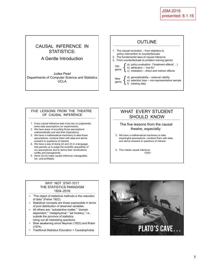
“The object of statistical methods is the reduction
f data” (Fisher 1922).
Statistical concepts are those expressible in terms
f joint distribution of observed variables.
All others are: “substantive matter,” “domain

dependent,” “metaphysical,” “ad hockery,” i.e.,

utside the province of statistics,

ruling out all interesting questions.

Slow awakening since Neyman (1923) and Rubin

(1974).

Traditional Statistics Education = Causalophobia

WHY NOT STAT-101? THE STATISTICS PARADIGM 1834–2016

JSM-2016 presented: 8.1.16

SLIDE 2

2 THE CAUSAL REVOLUTION

1. “More has been learned about causal inference in

the last few decades than the sum total of everything that had been learned about it in all prior recorded history.” (Gary King, Harvard, 2014)

2. From liability to respectability
JSM 2003 – 13 papers
JSM 2013 – 130 papers
3. The gems – for Fun and Profit
Its fun to solve problems that Pearson, Fisher,

Neyman, and my professors . . . were not able to articulate.

Problems that users pay for.

TRADITIONAL STATISTICAL INFERENCE PARADIGM

Data Inference Q(P) (Aspects of P) e.g., Infer whether customers who bought product A would also buy product B. Q = P(B | A) Joint Distribution

P

e.g., Estimate P′(sales) if we double the price. How does P change to P′? New oracle e.g., Estimate P′(cancer) if we ban smoking.

FROM STATISTICAL TO CAUSAL ANALYSIS:

1. THE DIFFERENCES

Data Inference Q(P′) (Aspects of P′) change Joint Distribution

P

Joint Distribution

P′

What remains invariant when P changes say, to satisfy P′(price=2)=1 Data Inference Q(P′) (Aspects of P′) change Note: P′(sales) ≠ P (sales | price = 2) e.g., Doubling price ≠ seeing the price doubled. P does not tell us how it ought to change.

FROM STATISTICAL TO CAUSAL ANALYSIS:

1. THE DIFFERENCES

Joint Distribution

P

Joint Distribution

P′

What happens when P changes? e.g., Estimate the probability that a customer who bought A would buy A if we were to double the price.

FROM STATISTICS TO COUNTERFACTUALS: RETROSPECTION

Data Inference Q(P′) (Aspects of P′) change Joint Distribution

P

Joint Distribution

P′

utcome

dependent Data Inference Q(M) (Aspects of M) Data Generating Model M – Invariant strategy (mechanism, recipe, law, protocol) by which Nature assigns values to variables in the analysis. Joint Distribution

STRUCTURAL CAUSAL MODEL THE NEW ORACLE

M

P – model of data, M – model of reality

P

SLIDE 3

3

WHAT KIND OF QUESTIONS SHOULD THE NEW ORACLE ANSWER THE CAUSAL HIERARCHY

(What is?) (What if?) (Why?) P(y | A) P(y | do(A)) P(yA’ | A)

SYNTACTIC DISTINCTION

Observational Questions:

“What if we see A”

Action Questions:

“What if we do A?”

Counterfactuals Questions:

“What if we did things differently?”

Options:

“With what probability?”

WHAT KIND OF QUESTIONS SHOULD THE NEW ORACLE ANSWER THE CAUSAL HIERARCHY

Observational Questions:

“What if we see A”

Action Questions:

“What if we do A?”

Counterfactuals Questions:

“What if we did things differently?”

Options:

“With what probability?” Bayes Networks Causal Bayes Networks Functional Causal Diagrams GRAPHICAL REPRESENTATIONS

FROM STATISTICAL TO CAUSAL ANALYSIS:

2. THE SHARP BOUNDARY

CAUSAL Spurious correlation Randomization / Intervention “Holding constant” / “Fixing” Confounding / Effect Instrumental variable Ignorability / Exogeneity ASSOCIATIONAL Regression Association / Independence “Controlling for” / Conditioning Odds and risk ratios Collapsibility / Granger causality Propensity score

1. Causal and associational concepts do not mix. 2. 3. 4. 4. Non-standard mathematics: a) Structural equation models (Wright, 1920; Simon, 1960) b) Counterfactuals (Neyman-Rubin (Yx), Lewis (x Y))

ASSOCIATIONAL Regression Association / Independence “Controlling for” / Conditioning Odds and risk ratios Collapsibility / Granger causality Propensity score

1. Causal and associational concepts do not mix. 3. Causal assumptions cannot be expressed in the mathematical language of standard statistics.

FROM STATISTICAL TO CAUSAL ANALYSIS:

3. THE MENTAL BARRIERS

2. No causes in – no causes out (Cartwright, 1989) causal conclusions

⇒

}

data causal assumptions (or experiments)

CAUSAL Spurious correlation Randomization / Intervention “Holding constant” / “Fixing” Confounding / Effect Instrumental variable Ignorability / Exogeneity

17

C (Climate) R (Rain) S (Sprinkler) W (Wetness) Graph (G) Model (M) C = fC(UC ) S = fS(C,US) R = fR(C,UR) W = fW (S,R,UW )

A MODEL AND ITS GRAPH

C (Climate) R (Rain) S (Sprinkler) W (Wetness) Graph (G) Model (M) Would the pavement be wet HAD the sprinkler been ON?

DERIVING COUNTERFACTUALS FROM A MODEL

C = fC(UC ) S = fS(C,US) R = fR(C,UR) W = fW (S,R,UW )

SLIDE 4

4

C (Climate) R (Rain) S = 1 (Sprinkler) W (Wetness)

DERIVING COUNTERFACTUALS FROM A MODEL

Graph (G) C = fC(UC ) S = 1 R = fR(C,UR) W = fW (S,R,UW ) Mutilated Model (MS=1)

Would the pavement be wet had the sprinkler been ON? Find if W = 1 in MS=1 Find if fW (S = 1, R, UW) = 1 or WS = 1 = 1 What is the probability that we find the pavement is wet if we turn the sprinkler ON? Find if P(WS = 1 = 1) = P(W = 1 | do(S = 1))

C (Climate) R (Rain) S = 1 (Sprinkler) W (Wetness)

DERIVING COUNTERFACTUALS FROM A MODEL

Graph (G) C = fC(UC ) S = 1 R = fR(C,UR) W = fW (S,R,UW ) Mutilated Model (MS=1)

Would it rain if we turn the sprinkler ON? Not necessarily, because RS = 1 = R

C (Climate) R = 1 (Rain) S = 1 (Sprinkler) W (Wetness)

DERIVING COUNTERFACTUALS FROM A MODEL

Graph (G) KNIFE CUTTING Would the pavement be wet had the rain been ON? Find if W = 1 in MR=1

Find if fW (S, R = 1, UW) = 1 EVERY COUNTERFACTAUL HAS A VALUE IN M

Mutilated Model (MR=1) C = fC(UC ) S = fS(C,US) R = 1 W = fW (S,R,UW )

THE TWO FUNDAMENTAL LAWS OF CAUSAL INFERENCE

1. The Law of Counterfactuals (and Interventions)

(M generates and evaluates all counterfactuals.) and all interventions

Yx(u) = YMx (u)

ATE = Eu[Yx(u)] = E[Y | do(x)]

THE TWO FUNDAMENTAL LAWS OF CAUSAL INFERENCE

1. The Law of Counterfactuals (and Interventions)

(M generates and evaluates all counterfactuals.)

2. The Law of Conditional Independence (d-separation)

(Separation in the model ⇒ independence in the distribution.)

Yx(u) = YMx (u) (X sep Y | Z)G(M ) ⇒ (X ⊥ ⊥ Y | Z)P(v)

C (Climate) R (Rain) S (Sprinkler) W (Wetness)

THE LAW OF CONDITIONAL INDEPENDENCE

Graph (G) Model (M) Gift of the Gods If the U 's are independent, the observed distribution P(C,R,S,W) satisfies constraints that are: (1) independent of the f 's and of P(U), (2) readable from the graph. C = fC(UC ) S = fS(C,US) R = fR(C,UR) W = fW (S,R,UW )

SLIDE 5

5

S ⊥ ⊥ R | C e.g., C ⊥ ⊥ W | (S,R)

D-SEPARATION: NATURE’S LANGUAGE

FOR COMMUNICATING ITS STRUCTURE

Every missing arrow advertises an independency, conditional

n a separating set.

Applications:

1. Model testing
2. Structure learning
3. Reducing "what if I do" questions to symbolic calculus
4. Reducing scientific questions to symbolic calculus

C (Climate) R (Rain) S (Sprinkler) W (Wetness) Graph (G) Model (M) C = fC(UC ) S = fS(C,US) R = fR(C,UR) W = fW (S,R,UW )

ELIMINATING CONFOUNDING BIAS THE BACK-DOOR CRITERION

P(y | do(x)) is estimable if there is a set Z of variables that if conditioned on, would block all X-Y paths that are severed by the intervention and none other. Z3 Z2 Z5 Z1 X = x Z4 Z6 Y Z3 Z2 Z5 Z1 X = x Z4 Z6 Y Z do(x)-intervention do(x)-emulation

Moreover, P(y | do((x)) = P(y | x,z)P(z)

z

∑

(Adjustment) Back-door =⇒ Yx ⊥ ⊥ X | Z =⇒ (Y ⊥ ⊥ X | Z)GX

WHAT IF VARIABLES ARE UNOBSERVED? EFFECT OF WARM-UP ON INJURY (Shrier & Platt, 2008)

No, no! ATE = ✔ ETT = ✔ PNC = ✔

GOING BEYOND ADJUSTMENT

Smoking Tar Cancer Genotype (Unobserved)

Goal: Find the effect of Smoking on Cancer, P(c | do(s)), given samples from P(S, T, C), when latent variables confound the relationship S-C. Query Data

Smoking Tar Cancer

Genotype (Unobserved)

P (c | do(s))

Query Estimand

IDENTIFICATION REDUCED TO CALCULUS (THE ENGINE AT WORK)

P(y | do(x),z,w) = P(y | do(x),w), P(y | do(x),do(z),w) = P(y | do(x),z,w), P(y | do(x),do(z),w) = P(y | do(x),w),

The following transformations are valid for every interventional distribution generated by a structural causal model M:

DO-CALCULUS

(THE WHEELS OF THE ENGINE)

Rule 1: Ignoring observations Rule 2: Action/observation exchange Rule 3: Ignoring actions

if (Y ⊥ ⊥ Z | X,W )GX if (Y ⊥ ⊥ Z | X,W )GXZ if (Y ⊥ ⊥ Z | X,W )GXZ(W )

SLIDE 6

6

Q = P(y1,y2,...,yn | do(x1,x2,...,xm),z1,z2,...,zk )

GEM 1: THE IDENTIFICATION PROBLEM IS SOLVED (NONPARAMETRICALLY)

The estimability of any expression of the form

can be decided in polynomial time.

If Q is estimable, then its estimand can be derived in

polynomial time.

The algorithm is complete.
Same for ETT (Shpitser 2008).

PROPENSITY SCORE ESTIMATOR (Rosenbaum & Rubin, 1983)

Z6 Z3 Z2 Z5 Z1 X Y Z4 Adjustment for e (z) replaces Adjustment for Z Theorem:

P(y | do(x)) = ?

e Can e replace {Z1, Z2, Z3, Z4, Z5} ?

e(z1,z2,z3,z4,z5) Δ = P(X = 1| z1,z2,z3,z4,z5) P(y | z,x)P(z) = P(y | e,x)P(e)

e

∑

z

∑

33

WHAT PROPENSITY SCORE (PS) PRACTITIONERS NEED TO KNOW

1. The asymptotic bias of PS is EQUAL to that of ordinary

adjustment (for same Z).

2. Including an additional covariate in the analysis CAN

SPOIL the bias-reduction potential of PS.

3. In particular, instrumental variables tend to amplify bias.
4. Choosing sufficient set for PS, requires causal knowledge,

which PS alone cannot provide. Z X Y X Y X Y Z X Y Z Z

e(z) = P(X = 1| Z = z) P(y | z,x)P(z) = P(y | e,x)P(e)

e

∑

z

∑

DAGS VS. POTENTIAL COUTCOMES AN UNBIASED PERSPECTIVE

1. Semantic Equivalence
2. Both are abstractions of Structural Causal

Models (SCM).

Yx(u) = YM x (u) X → Y y = f (x,z,u)

Yx(u) = All factors that affect Y when X is held

constant at X=x. Zx(u) = Zyx(u), Xy(u) = Xzy(u) = Xz(u) = X(u), Yz(u) = Yzx(u), Zx ⊥ ⊥ {Yz, X}

1. English: Smoking (X), Cancer (Y), Tar (Z), Genotypes (U)

X Y Z U

testable? Not too friendly: Consistent?, complete?, redundant?, plausible?,

2. Potential

Outcome:

CHOOSING A LANGUAGE TO ENCODE ASSUMPTIONS

Zx(u) = Zyx(u), Xy(u) = Xzy(u) = Xz(u) = X(u), Yz(u) = Yzx(u), Zx ⊥ ⊥ {Yz, X}

2. Counterfactuals:
1. English: Smoking (X), Cancer (Y), Tar (Z), Genotypes (U)

X Y Z U

3. Structural:

x = f1(u,ε1) y = f3(z,u,ε3) z = f2(x,ε2) ε1 ⊥ ⊥ ε2 ⊥ ⊥ ε3 U Z X Y

CHOOSING A LANGUAGE TO ENCODE ASSUMPTIONS

SLIDE 7

7

Your Honor! My client (Mr. A) died BECAUSE

he used that drug.

GEM 2: ATTRIBUTION
Your Honor! My client (Mr. A) died BECAUSE

he used that drug.

Court to decide if it is MORE PROBABLE THAN

NOT that A would be alive BUT FOR the drug!

PN = P(alive{no drugs} | dead,drug) ≥ 0.50

GEM 2: ATTRIBUTION

CAN FREQUENCY DATA DETERMINE LIABILITY?

WITH PROBABILITY ONE
Combined data tell more that each study alone

1≤ PN ≤1

Sometimes:

40

1. To understand how Nature works
2. To comply with legal requirements
3. To predict the effects of new type of interventions:

Signal re-routing and mechanism deactivating, rather than variable fixing

GEM 3: MEDIATION WHY DECOMPOSE EFFECTS?

41

X M Y

LEGAL IMPLICATIONS OF DIRECT EFFECT

What is the direct effect of X on Y ? (m-dependent) (Qualifications) (Hiring) (Gender) Can data prove an employer guilty of hiring discrimination? Adjust for M? No! No!

CDE = E(Y|do(x1),do(m))− E(Y|do(x0),do(m))

CDE identification is completely solved

X M Y

(Qualifications) (Hiring) (Gender) Can data prove an employer guilty of hiring discrimination?

The Legal Definition: Find the probability that “the employer would have acted differently had the employee been of different sex and qualification had been the same.”

LEGAL DEFINITION OF DISCRIMINATION

SLIDE 8

8

43

m = f (x, u) y = g (x, m, u) X M Y

NATURAL INTERPRETATION OF AVERAGE DIRECT EFFECTS

Natural Direct Effect of X on Y: The expected change in Y, when we change X from x0 to x1 and, for each u, we keep M constant at whatever value it attained before the change. Note the 3-way symbiosis

E[Yx1M x0 −Yx0 ]

Robins and Greenland (1992) – Pearl (2001)

DE(x0,x1;Y )

44

m = f (x, u) y = g (x, m, u) X M Y

DEFINITION OF INDIRECT EFFECTS

Indirect Effect of X on Y: The expected change in Y when we keep X constant, say at x0, and let M change to whatever value it would have attained had X changed to x1. In linear models, IE = TE - DE

E[Yx0M x1 −Yx0 ] ) ; , ( 1 Y x x IE

No controlled indirect effect

45

POLICY IMPLICATIONS OF INDIRECT EFFECTS

f GENDER QUALIFICATION HIRING

What is the indirect effect of X on Y? The effect of Gender on Hiring if sex discrimination is eliminated.

X M Y IGNORE

Deactivating a link – a new type of intervention

THE MEDIATION FORMULAS IN UNCONFOUNDED MODELS

X M Y

Fraction of responses explained by mediation (sufficient) Fraction of responses owed to mediation (necessary)

m = f (x, u1) y = g (x, m, u2) u1 independent of u2 TE − DE = DE = [E(Y | x1,m)− E(Y | x0,m)]P(m | x0)

m

∑

IE = [E(Y | x0,m)[P(m | x1)− P(m | x0)

m

∑

] TE = E(Y | x1)− E(Y | x0) IE = TE ≠ DE + IE

The nonparametric estimability of natural (and

controlled) direct and indirect effects can be determined in polynomial time given any causal graph G with both measured and unmeasured variables.

If NDE (or NIE) is estimable, then its estimand can be

derived in polynomial time.

The algorithm is complete and was extended to any

path-specific effects (Shpitser, 2013).

SUMMARY OF MEDIATION (GEM 3) Identification is a solved problem

W2 M Y T W3 M W2 Y T W3 M Y W2 T W3 M Y W2 T W3 (b) M Y W2 T W3 (a) M Y W2 T W3 (c) (e) (d) (f)

WHEN CAN WE IDENTIFY MEDIATED EFFECTS?

W1

SLIDE 9

9

W2 M Y T W3 M W2 Y T W3 M Y W2 T W3 M Y W2 T W3 (b) M Y W2 T W3 (a) M Y W2 T W3 (c) (e) (d) (f)

WHEN CAN WE IDENTIFY MEDIATED EFFECTS?

W1

The problem

How to combine results of several experimental

and observational studies, each conducted on a different population and under a different set of conditions,

so as to construct a valid estimate of effect size

in yet a new population, unmatched by any of those studied.

GEM 4: GENERALIZABILITY AND DATA FUSION

(b) New York

Survey data Resembling target

(c) Los Angeles

Survey data Younger population

(e) San Francisco

High post-treatment blood pressure

(d) Boston

Age not recorded Mostly successful lawyers

(f) Texas

Mostly Spanish subjects High attrition

(h) Utah

RCT, paid volunteers, unemployed

(g) Toronto

Randomized trial College students

(i) Wyoming

RCT, young athletes

THE PROBLEM IN REAL LIFE

Target population Query of interest: Q = P*(y | do(x))

(a) Arkansas

Survey data available

*

∏

X Y (f) Z W X Y (b) Z W X Y (c) Z S W X Y (a) Z W X Y (g) Z W X Y (e) Z W S S X Y (h) Z W X Y (i) Z S W S X Y (d) Z W

THE PROBLEM IN MATHEMATICS

Target population Query of interest: Q = P*(y | do(x))

*

∏

X Y (f) Z W X Y (b) Z W X Y (c) Z S W X Y (a) Z W X Y (g) Z W X Y (e) Z W S S X Y (h) Z W X Y (i) Z S W S X Y (d) Z W Target population Query of interest: Q = P*(y | do(x))

*

∏

THE SOLUTION IS IN ALGORITHMS

Experimental study in LA Measured:

P(x,y,z) P(y | do(x),z)

P*(y | do(x)) = ?

Observational study in NYC Measured: P*(x,y,z)

P*(z) ≠ P(z)

X (Intervention) Y (Outcome) Z (Age)

= P(y | do(x),z)P*(z)

z

∑

Π (LA) Π* (NY)

THE TWO–POPULATION PROBLEM

WHAT CAN EXPERIMENTS IN LA TELL US ABOUT NYC? Transport Formula: Q = F(P, Pdo, P*) Needed: Q =

SLIDE 10

10

X

TRANSPORT FORMULAS DEPEND ON THE CAUSAL STORY

a) Z represents age b) Z represents language skill c) Z represents a bio-marker

P(y | do(x)) = P(y | do(x),z)P(z)

z

∑

P*(y | do(x)) =

X Y Z (b) S (a) X Y (c) Z S

P(y | do(x)) P(y | do(x),z)P*(z| x )

z

∑

P*(y | do(x)) =

Y Z S Lesson: Not every dissimilarity deserves re-weighting.

TRANSPORTABILITY REDUCED TO CALCULUS

Theorem A causal relation R is transportable from Π to Π* if and

nly if it is reducible, using the rules of do-calculus,

to an expression in which S is separated from do( ).

R *

∏ ( )= P*(y | do(x)) = P(y | do(x),s)

= P(y | do(x),s,w)P(w | do(x),s)

w

∑

= P(y | do(x),w)P(w | s)

w

∑

= P(y | do(x),w)P*(w)

w

∑

X Y Z S W Query Estimand

S'

U W

RESULT: ALGORITHM TO DETERMINE IF AN EFFECT IS TRANSPORTABLE

X Y Z V S T

INPUT: Annotated Causal Graph OUTPUT:

1. Transportable or not?
2. Measurements to be taken in the

experimental study

3. Measurements to be taken in the

target population

4. A transport formula
5. Completeness (Bareinboim, 2012)

S Factors creating differences

P(y | do(x)) = P(y | do(x),z) P(z | w)

w

∑

z

∑

P(w | do(w),t)P*(t)

t

∑

X Y (f) Z S X Y (d) Z S W

WHICH MODEL LICENSES THE TRANSPORT OF THE CAUSAL EFFECT X→Y

(c) X Y Z S Y (e) Z S W Y Z S W X Y Z S W (b) Y X S (a) Y X S S External factors creating disparities

Yes Yes No Yes No Yes

SUMMARY OF TRANSPORTABILITY RESULTS

Nonparametric transportability of experimental

results from multiple environments can be determined provided that commonalities and differences are encoded in selection diagrams.

When transportability is feasible, the transport

formula can be derived in polynomial time.

The algorithm is complete.

GEM 5: RECOVERING FROM SAMPLING SELECTION BIAS

Transportability Selection Bias X (Treatment) Y (Outcome) Z (Age) S (Beach proximity) S = disparity-producing factors S = sampling mechanism S = 1 Z (Age) X (Treatment) Y (Outcome) Nature-made Man-made Non-estimable Non-estimable

SLIDE 11

11

Theorem: A query Q can be recovered from selection biased data iff Q can be transformed, using do-calculus to a form provided by the data, i.e., (i) All do-expressions are conditioned on S = 1 (ii) No do-free expression is conditioned on S = 1

RECOVERING FROM SELECTION BIAS

Query: Find P(y | do(x)) Data: P(y | do(x),z,S = 1) from study P(y,x,z) from survey

RECOVERING FROM SELECTION BIAS

Y Z X Example: S=1

P(y | do(x)) = P(y | do(x),z)P(z | do(x))

z

∑

= P(y | do(x),z)P(z | x)

z

∑

(Rule 2) = P(y | do(x),z,S = 1)P(z | x)

z

∑

(Rule 1)

GEM 6: MISSING DATA: A STATISTICAL PROBLEM TURNED CAUSAL

Sam- ple # X Y Z 1 1 2 1 1 3 1 m m 4 1 m 5 m 1 m 6 m 1 7 m m 8 1 m 9 m 10 1 m 11 1 1

Question:

Is there a consistent estimator of P(X,Y,Z)? That is, is P(X,Y,Z) estimable (asymptotically) as if no data were missing. Conventional Answer: Run imputation algorithm and, if missingness occurs at random (MAR), (a condition that is untestable and uninterpretable), then it will coverage to a consistent estimate.

GEM 6: MISSING DATA: A STATISTICAL PROBLEM TURNED CAUSAL

Sam- ple # X Y Z 1 1 2 1 1 3 1 m m 4 1 m 5 m 1 m 6 m 1 7 m m 8 1 m 9 m 10 1 m 11 1 1

Question:

Is there a consistent estimator of P(X,Y,Z)? That is, is P(X,Y,Z) estimable (asymptotically) as if no data were missing. Model-based Answers:

1. There is no Model-free estimator, but,
2. Given a missingness model, we can tell

you yes/no, and how.

3. Given a missingness model, we can tell

you whether or not it has testable implications.

SMART ESTIMATION OF P(X,Y,Z)

Example 1: P(X,Y,Z) is estimable Rz Ry Rx Z X Y P(X,Y,Z) = P(Z | X,Y,Rx = 0,Ry = 0,Rz = 0) P(X |Y,Rx = 0,Ry = 0) P(Y | Ry = 0)

Sam- ple # X Y Z 1 1 2 1 1 3 1 m m 4 1 m 5 m 1 m 6 m 1 7 m m 8 1 m 9 m 10 1 m 11 1 1

Rx = 0 ⇒ X observed

Rx = 1 ⇒ X missing Testable implications:

Z ⊥ ⊥ Ry | Rz = 0 Rz ⊥ ⊥ Rx |Y,Ry = 0

SMART ESTIMATION OF P(X,Y,Z)

Example 1: P(X,Y,Z) is estimable Rz Ry Rx Z X Y P(X,Y,Z) = P(Z | X,Y,Rx = 0,Ry = 0,Rz = 0) P(X |Y,Rx = 0,Ry = 0) P(Y | Ry = 0)

Sam- ple # X Y Z 1 1 2 1 1 3 1 m m 4 1 m 5 m 1 m 6 m 1 7 m m 8 1 m 9 m 10 1 m 11 1 1

Rx = 0 ⇒ X observed

Rx = 1 ⇒ X missing Testable implications:

X ⊥ ⊥ Rx | Y is not testable

because X is not fully observed.

SLIDE 12

12 SMART ESTIMATION OF P(X,Y,Z)

Example 1: P(X,Y,Z) is estimable Example 2: P(X,Y,Z) is non-estimable Rz Ry Rx Z X Y Rz Ry Rx Z X Y P(X,Y,Z) = P(Z | X,Y,Rx = 0,Ry = 0,Rz = 0) P(X |Y,Rx = 0,Ry = 0) P(Y | Ry = 0)

Sam- ple # X Y Z 1 1 2 1 1 3 1 m m 4 1 m 5 m 1 m 6 m 1 7 m m 8 1 m 9 m 10 1 m 11 1 1

Rx = 0 ⇒ X observed

Rx = 1 ⇒ X missing

WHAT MAKES MISSING DATA A CAUSAL PROBLEM?

The knowledge required to guarantee consistency is causal i.e., it comes from our understanding of the mechanism that causes missingness (not from hopes for fortunate conditions to hold). Graphical models of this mechanism provide:

1. Tests for MCAR and MAR,
2. consistent estimates for large classes of MNAR,
3. testable implications of missingness models,
4. closed-form estimands, bounds, and more.
5. Query-smart estimation procedures.

CONCLUSIONS

A revolution is judged by the gems it spawns.
Each of the six gems of the causal revolution is

shining in fun and profit.

More will be learned about causal inference in

the next decade than most of us imagine today.

Because statistical education is about to catch