Bayes rule recall def of conditional: P(a|b) = P(a^b) / P(b) if - - PDF document

Geoff Gordon—10-701 Machine Learning—Fall 2013

Bayes rule

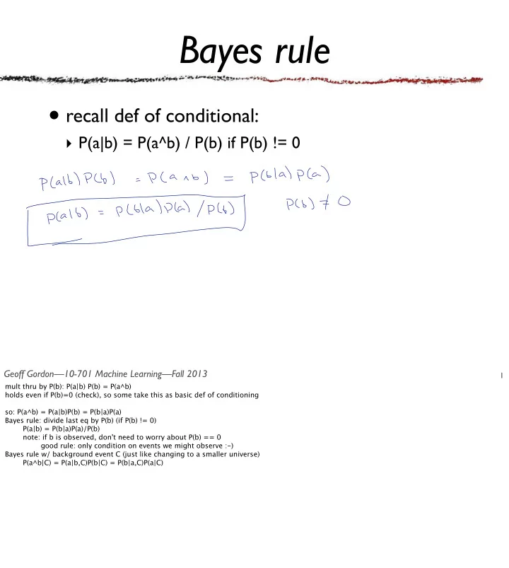
• recall def of conditional:
• P(a|b) = P(a^b) / P(b) if P(b) != 0

1

• mult thru by P(b): P(a|b) P(b) = P(a^b)

holds even if P(b)=0 (check), so some take this as basic def of conditioning so: P(a^b) = P(a|b)P(b) = P(b|a)P(a) Bayes rule: divide last eq by P(b) (if P(b) != 0) P(a|b) = P(b|a)P(a)/P(b) note: if b is observed, don't need to worry about P(b) == 0 good rule: only condition on events we might observe :-) Bayes rule w/ background event C (just like changing to a smaller universe) P(a^b|C) = P(a|b,C)P(b|C) = P(b|a,C)P(a|C)

Geoff Gordon—10-701 Machine Learning—Fall 2013

Bayes rule: sum version

• P(a | b) = P(b | a) P(a) / P(b)

2

what if we don't know P(b), but still know P(b|a) and P(a) (often happens) suppose MEEP A = a1, a2, ..., an for moderate n we know sum_i P(ai | b) = 1 so sum_i P(ai | b) P(b) = P(b) (mult by P(b) on both sides) LHS is sum_i P(b|ai) P(ai) (another application of Bayes rule) each term assumed known, sum tractable since n moderate

Geoff Gordon—10-701 Machine Learning—Fall 2013

Bayes rule in ML

• P(model | data) = P(data | model) P(model) / P(data)

3

Why do we care about Bayes? Lets us take info about conditional in one direction (P(data | model)) and get info about the other direction (P(model| data)). LHS P(model|data) tells us which models are probable give the data. This is (mostly) what we want out of ML! Called “posterior” P(data | model) usually has an explicit formula, e.g., gaussian distribution: P(x_i|mu) = exp(-(x_i-mu)^2/2)/√2pi). Called “likelihood” P(model) = “prior” -- sometimes controversial but not hard to write a minimally reasonable one P(data): “normalizing constant” (also “annoyance”) -- often hard to get can use sum version of Bayes rule (sum numerator over models) OK if not too many models under consideration can use sum version + approximation tricks (numerical quadrature, MCMC like Gibbs) another idea on next slide note: normalizing constants are often ignored. This is a common pattern, but it doesn’t mean it’s always safe (or a good idea) to ignore them! Sometimes all of the useful information is in the normalizing constant...

Geoff Gordon—10-701 Machine Learning—Fall 2013

Bayes rule vs. MAP vs. MLE

• P(model | data) = P(data | model) P(model) / P(data)

4

MAP: just take model for which RHS is highest -- if we have to choose just one point from posterior density, why not this one? [sketch] now P(data) really is ignorable (doesn’t change order) Seems like a horrible approximation (from Bayesian perspective), but actually has theory to back it up. MLE: ignore P(model) term too. Why? Because people argue about the prior; because with enough evidence from data it might become negligible. Seems even worse, but still has theory to back it up. (see next slide)

Geoff Gordon—10-701 Machine Learning—Fall 2013

Jerzy Neyman

Frequentist vs. Bayes

• Nature as adversary vs. Nature as probability

distribution

• Probability as long-run frequency of repeatable

events vs. odds for bets I'm willing to take

5

rev. Thomas Bayes

FIGHT!!!

see also: http://www.xkcd.com/1132/

treat Nature as a probability distribution vs. an adversary Bayes: if you have the right distribution over models and can compute with it, good things happen Frequentist: but both of those are horrible assumptions Plenty of paradoxes for both sides if you want to cast stones

Geoff Gordon—10-701 Machine Learning—Fall 2013

Test for a rare disease

• About 0.1% of all people are infected
• Test detects all infections
• Test is highly specific: 1% false positive
• You test positive. What is the probability you have

the disease?

6

P(disease) P(test | +disease) P(test | -disease) P(+disease | +test) = P(+test | +disease) P(+disease) / P(+test) P(+t) = P(+t|+d)P(+d) + P(+t|-d)P(-d) = 1 * .001 / (1*.001 + .01*.999) = .091

Geoff Gordon—10-701 Machine Learning—Fall 2013

Test for a rare disease

• About 0.1% of all people are infected
• Test detects all infections
• Test is highly specific: 1% false positive
• You test positive. What is the probability you have

the disease?

6

Bonus: what is probability an average med student gets this question wrong?

P(disease) P(test | +disease) P(test | -disease) P(+disease | +test) = P(+test | +disease) P(+disease) / P(+test) P(+t) = P(+t|+d)P(+d) + P(+t|-d)P(-d) = 1 * .001 / (1*.001 + .01*.999) = .091

Geoff Gordon—10-701 Machine Learning—Fall 2013

Follow-up test

• Test 2: detects 90% of infections, 5% false positives
• P(+disease | +test1, +test2) =

7

P(+disease | +test1, +test2) = P(+1, +2 | +d) P(+d) / P(+1, +2) P(+12) = P(+12|+d)P(+d) + P(+12|-d)P(-d) = 1*.9*.001 / (1*.9*.001 + .05*.01*.999) = .643 Test 1 seems better than test 2 -- why not use test 1 twice? A: T1 is conditionally independent of T2 given disease state -- probably not true for T1 w/ itself

Geoff Gordon—10-701 Machine Learning—Fall 2013

Independence

8

for events: defined as P(a^b) = P(a)P(b), like rows/cols of checkerboard P(~a^b) = P(b) – P(a^b) = P(b) - P(a)P(b) = (1-P(a))P(b) = P(~a)P(b) for r.v.s: P(A,B) = P(A)P(B) shorthand: joint probability table = outer product of marginal probability tables P(A=a_i ^ B=b_i) = P(A=a_i) P(B=b_i) intuition: knowing a or ~a tells us nothing about B Bayes rule version: P(A) = P(A|B) i.e., P(A=a_i) = P(A=a_i | B=b_j) for all a_i, b_j w/ P(B=b_j > 0) follows: P(a|b) = P(a^b)/P(b) = P(a)P(b)/P(b) = P(a), as long as P(b)!=0 some take this as definition of independence

Geoff Gordon—10-701 Machine Learning—Fall 2013

Conditional independence

9

conditional independence: X _|_ Y | Z if, for all values of z_i, P(X,Y|z_i)=P(X|z_i)P(Y|z_i) i.e., after we condition on z_i, X and Y are independent P(x, y | z) = P(x | z) P(y | z) for any values xyz of XYZ this is a statement about a 3d table and two 2d tables

London taxi drivers: A survey has pointed out a positive and

significant correlation between the number of accidents and wearing

• coats. They concluded that coats could hinder movements of drivers and

be the cause of accidents. A new law was prepared to prohibit drivers from wearing coats when driving. Finally another study pointed out that people wear coats when it rains…

Conditionally Independent

slide credit: Barnabas

Geoff Gordon—10-701 Machine Learning—Fall 2013

humor credit: xkcd

More on the importance of conditioning

11

Geoff Gordon—10-701 Machine Learning—Fall 2013

Samples

12

…

i.i.d. sample of an r.v.: N independent copies of the same checkerboard sample is itself an r.v. in a bigger space (a 2N-dim hypercheckerboard) atomic events are tuples of original atomic events sample (r.v.) vs. population (the One True checkerboard) statistic = any function of the sample

• usu. order-independent (symmetric) but doesn't have to be

statistics are r.v.s e.g., sample mean, variance goal of statistics (big or small S): use statistics to find out something about the population

Geoff Gordon—10-701 Machine Learning—Fall 2013

Recall: spam filtering

13

classification problem: given data (x_i, y_i) N pairs, x_i \in {0,1}^d, y_i \in {0,1} -- write x_i = (x_{i1} .. x_{id}) produce rule which goes from future x -> predicted y e.g.: spam filtering: x_ij = presence of word i in doc j bag of words

Geoff Gordon—10-701 Machine Learning—Fall 2013

Bag of words

14

Geoff Gordon—10-701 Machine Learning—Fall 2013

A ridiculously naive assumption

• Assume:
• Clearly false:
• Given this assumption, use Bayes rule

15

assumption: x_{ij} _|_ x_{ik} | c_i for all j,k \in 1..d, j != k clearly false: "CMU" not independent of "Bayes" given this "naive" assumption, use "Bayes" rule

Geoff Gordon—10-701 Machine Learning—Fall 2013

Graphical model

16

spam x1 x2

. . .

xn

spam xi

i=1..n

arrows spam-> xi say xi depends on spam lack of other arrows into xi: the xi’s are conditionally independent given spam “macro” or “for loop” shorthand: called a “plate model”

Geoff Gordon—10-701 Machine Learning—Fall 2013

Naive Bayes

• P(spam | email ∧ award ∧ program ∧ for ∧ internet

∧ users ∧ lump ∧ sum ∧ of ∧ Five ∧ Million)

17

P(spam | email award program for internet users lump sum of Five Million) = P(email ... Million | spam) P(spam) / [P(email ... Million | spam) P(spam) + P(email ... Million | not-spam) P(~spam)] (sum version of Bayes rule) = P(email | spam) P(award | spam) ... P(Million | spam) P(spam) / [ "" | spam + "" | ~spam] (independence assumption) suppose we know P(word j | spam) and P(word j | ~spam) for all j and suppose we know P(spam) and P(~spam) how? see slightly later then above is easy to calculate! now keep messages w/ P(spam) < threshold adjust threshold based on user preference: chance of missing internet lottery win vs. wants to get work done

Geoff Gordon—10-701 Machine Learning—Fall 2013

In log space

zspam = ln(P(email | spam) P(award | spam) ... P(Million | spam) P(spam)) z~spam = ln(P(email | ~spam) ... P(Million | ~spam) P(~spam))

18

z_spam = ln(P(email | spam) P(award | spam) ... P(Million | spam) P(spam)) z_~spam = ln(P(email | ~spam) P(award | ~spam) ... P(Million | ~spam) P(~spam)) result is then P(spam | ... ) = exp(z_spam) / [exp(z_spam) + exp(z_~spam)] = 1 / [1 + exp(z_~spam - z_spam)] = 1 / [1 + exp(-z)] where z = z_spam - z_~spam sigmoid or logistic function (sketch): logit(z) big z: confident in spam big -z: confident in ~spam

Geoff Gordon—10-701 Machine Learning—Fall 2013

Collect terms

zspam = ln(P(email | spam) P(award | spam) ... P(Million | spam) P(spam)) z~spam = ln(P(email | ~spam) ... P(Million | ~spam) P(~spam)) z = zspam – zspam

19

= ln P(spam) - ln(P(~spam)) <-- call this b + ln P(email | spam) - ln P(email | ~spam) <-- call this w_{email} + ln P(award | spam) - ln P(award | ~spam) <-- w_{award} + ... sum is over words in our message i.e.: to classify message x_i, compute b + sum_{j\in vocabulary} w_j x_{ij} (x_{ij} = 0 when word j not in message) threshold on result: b + sum_j w_j x_{ij} >= 0 "linear discriminant" "decision boundary" : b + sum_j w_j x_{ij} = 0

Geoff Gordon—10-701 Machine Learning—Fall 2013

Linear discriminant

20

threshold on result: b + sum_j w_j x_{ij} >= 0 "linear discriminant" "decision boundary" : b + sum_j w_j x_{ij} = 0

Geoff Gordon—10-701 Machine Learning—Fall 2013

Intuitions

21

word of warning: nominally, P(spam) is logit(z) really, logit(z) usually close to 0 or 1 even in marginal cases why? [failure of independence assumption] fix: use logit(eps*z) for appropriately-chosen eps (***) what are highly useful/discriminative words? log(P(word j|spam)/P(word j|~spam)) far from zero i.e., really low probability one class, moderate to high in the other (since log is much more sensitive near 0) but decent chance of actually seeing word j suggested measure: P(j)log(P(j|s)/P(j|~s)) -- looks like KL / relative entropy! eg: "lottery" really low in legit emails -- not high in spam, but significantly nonzero

Geoff Gordon—10-701 Machine Learning—Fall 2013

How to get probabilities?

22

How to get the needed probabilities? flip coin, count heads or tails 3H, 7T: estimate P(H)=.3 what if 0H, 2T? hard zero probability seems bad Hack: estimate P(H) = (#H+0.5)/(#H+#T+1) here, 0.5/3 = 1/6: pretty sure but not hard zero turns out not to be a hack after all… called "Laplace smoothing", MAP for Dirichlet prior for words, sample count: might expect it to be proportional to population prob estimator: count(word)/(total # words) e.g., if we see "avocado" 10 times in 100k words, estimate P(avocado) = 1/10k count 0: e.g., "syzygy" not in training set but appears in test doc get log(0)=-infty in answer, bad. estimate p(word) as (lambda+count(word))/(lambda*words + total#words) small lambda > 0

Geoff Gordon—10-701 Machine Learning—Fall 2013

Improvements

23

n-grams, character string features, treat (multiple) headers vs. body difgerently, features of attachments, take account of body length, generalize among words using edit distance, stemming, POS-tagging, parsing, named entity resolution, collaborative spam-filters (if everyone's winning the lottery...), soft whitelists/blacklists (of domains, IP addresses, senders), ... general rule: most important part of practical ML is to think of good sources of information, then figure out how to get algorithm to pay attention to them

Geoff Gordon—10-701 Machine Learning—Fall 2013

Perceptron

24

classification again: X = ((x1, y1) .. (xN, yN)) yi \in {-1, 1} <-- instead of 0/1 for convenience assume x_ij in {0,1} if desired, but works just as well w/ \Re^d ex: spam filtering, or digit classific'n

Geoff Gordon—10-701 Machine Learning—Fall 2013

Digit recognition

25

digit recognition: x_{ij} = pixel j intensity in image i classify (say) 4 vs 9

Geoff Gordon—10-701 Machine Learning—Fall 2013

Linear separability

26

linear discriminant: z_i = x_i \cdot w + b (note notation change: x_i\cdot w = \sum_j x_ij w_j; Alex wrote <xi,w>) z_i > 0 when y_i = +1 z_i < 0 when y_i = -1 i.e., no errors and nothing on decision boundary suppose data set X is separable; how can we find w in this case?

Geoff Gordon—10-701 Machine Learning—Fall 2013

Simplify notation

27

simplify notation: homogeneous rep: xi \in \Re^d assume last component x_{id} = 1 in all examples if not, set d := d+1 and just append 1 to every example now, add b to last component of w: say w = w_old + [0 0 0 ... b] x_i \cdot w = x_i\cdot (w_old + [0 0 0 ... b]) = x_i \cdot w_old + b = z_i benefit: don't need b in our notation any more flip -ves: write ui = yi xi \in \Re^n x_i \cdot w > 0 when y_i = +1 ==> u_i \cdot w > 0 x_i \cdot w < 0 when y_i = -1 ==> u_i \cdot w > 0 so now, just write u_i \cdot w > 0 for all i

Geoff Gordon—10-701 Machine Learning—Fall 2013

First algorithm: LP

28

LP: we have a system of linear inequalities almost an LP -- if it were, we'd be done (hand it to CPLEX and go for cofgee) but our ineqs are strict (LP software requires >= not >) suppose we know eps = min_i u_i\cdot w now we can write u_i\cdot w >= eps for all i but we don't know eps -- trick: let v = w/eps now u_i\cdot v >= 1 for all i solve for v -- and eps doesn't matter remember this algorithm: we’ll see another one like it when we get to support vector machines

Geoff Gordon—10-701 Machine Learning—Fall 2013

#2: the “perceptron algorithm”

29

ui · w > 0 ∀i

simple algorithm: start at w = 0 pick a random training point ui = yi xi if inequality is satisfied, great if not, w := w + ui ui . w_new = ui . w + ui . ui > ui . w closer to satisfying ineq repeat This algorithm was implemented in 1958 on the “Mark I Perceptron”, which represented weights with variable resistors (i.e., dimmer switches), and used motors to turn the knobs for the update (!) To analyze: draw a sphere around all ui. (For convenience suppose radius 1; if not, renorm.) Margin gamma: max_{||w|| <= 1} min_i u_i . w (draw it)

Geoff Gordon—10-701 Machine Learning—Fall 2013

Perceptron proof

30 suppose w* (unknown) separates w/ margin gamma, ||w*||=1 On every update, w_new . w* = (w + ui) . w* = w . w* + ui . w* >= w . w* + gamma So, after T mistakes, w . w* >= T gamma (starts at 0, increases by gamma each time) w_new . w_new = (w + ui) . (w + ui) = w . w + 2 w . ui + ui . ui <= w . w + 1 So, after T mistakes, w . w <= T T gamma <= w . w* <= ||w|| ||w*|| (Cauchy-Schwartz) = sqrt(w.w) <= sqrt(T) divide thru by sqrt T and by gamma: sqrt(T) <= 1/gamma