Chapter 4 Chapter 4 The Fourier Series and The Fourier Series and - - PDF document

Chapter 4 The Fourier Series and Fourier Transform Chapter 4 The Fourier Series and Fourier Transform

• Let x(t) be a CT periodic signal with period

T, i.e.,

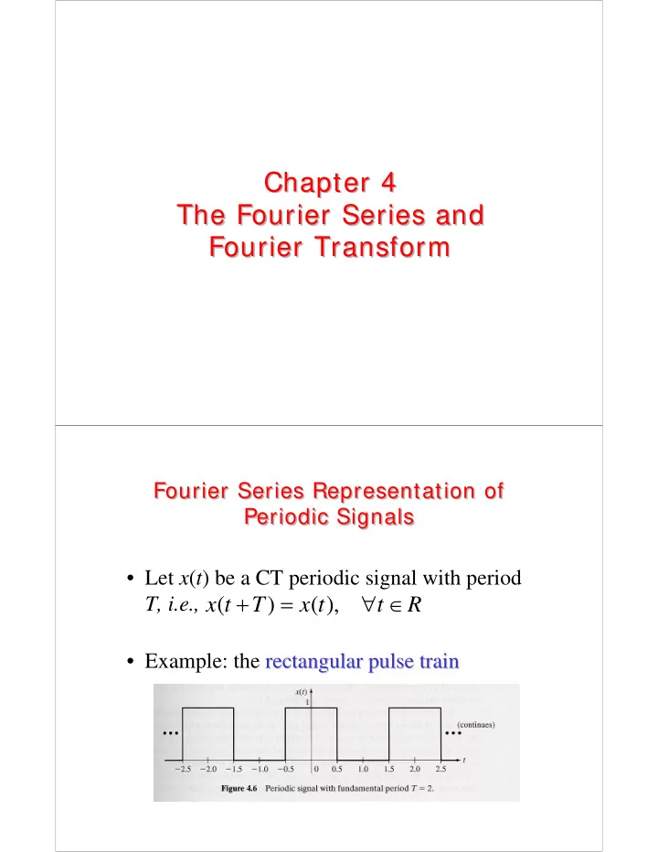
• Example: the rectangular pulse train

rectangular pulse train Fourier Series Representation of Periodic Signals Fourier Series Representation of Periodic Signals

( ) ( ), x t T x t t R + = ∀ ∈

• Then, x(t) can be expressed as

where is the fundamental fundamental frequency frequency (rad/sec) of the signal and The Fourier Series The Fourier Series

( ) ,

jk t k k

x t c e t

ω ∞ =−∞

= ∈

∑

• / 2

/ 2

1 ( ) , 0, 1, 2,

• T

jk t k T

c x t e dt k T

ω − −

= = ± ±

∫

… 2 /T ω π =

is called the constant or dc component of x(t)

c

• A periodic signal x(t), has a Fourier series

if it satisfies the following conditions:

• 1. x(t) is absolutely

absolutely integrable integrable over any period, namely

• 2. x(t) has only a finite number of maxima

finite number of maxima and minima and minima over any period

• 3. x(t) has only a finite number of

finite number of discontinuities discontinuities over any period Dirichlet Conditions Dirichlet Conditions

| ( ) | ,

a T a

x t dt a

+

< ∞ ∀ ∈

∫

• From figure , so
• Clearly x(t) satisfies the Dirichlet conditions and

thus has a Fourier series representation

Example: The Rectangular Pulse Train Example: The Rectangular Pulse Train

2 T = 2 / 2 ω π π = =

Example: The Rectangular Pulse Train – Cont’d Example: The Rectangular Pulse Train – Cont’d

|( 1)/ 2|

1 1 ( ) ( 1) , 2

k jk t k k odd

x t e t k

π

π

∞ − =−∞

= + − ∈

∑

• By using Euler’s formula, we can rewrite

as as long as x(t) is real

• This expression is called the trigonometric

trigonometric Fourier series Fourier series of x(t) Trigonometric Fourier Series Trigonometric Fourier Series

( ) ,

jk t k k

x t c e t

ω ∞ =−∞

= ∈

∑

• 1

( ) 2 | |cos( ),

k k k

x t c c k t c t ω

∞ =

= + + ∠ ∈

∑

• dc component

dc component k k-

• th

th harmonic harmonic

• The expression

can be rewritten as Example: Trigonometric Fourier Series of the Rectangular Pulse Train Example: Trigonometric Fourier Series of the Rectangular Pulse Train

|( 1)/ 2|

1 1 ( ) ( 1) , 2

k jk t k k odd

x t e t k

π

π

∞ − =−∞

= + − ∈

∑

• (

1)/ 2 1

1 2 ( ) cos ( 1) 1 , 2 2

k k k odd

x t k t t k π π π

∞ − =

⎛ ⎞ ⎡ ⎤ = + + − − ∈ ⎜ ⎟ ⎣ ⎦ ⎝ ⎠

∑

• Given an odd positive integer N, define the

N-th partial sum of the previous series

• According to Fourier

Fourier’ ’s theorem s theorem, it should be Gibbs Phenomenon Gibbs Phenomenon

( 1)/ 2 1

1 2 ( ) cos ( 1) 1 , 2 2

N k N k k odd

x t k t t k π π π

− =

⎛ ⎞ ⎡ ⎤ = + + − − ∈ ⎜ ⎟ ⎣ ⎦ ⎝ ⎠

∑

• lim |

( ) ( ) | 0

N N

x t x t

→∞

− =

Gibbs Phenomenon – Cont’d Gibbs Phenomenon – Cont’d

3( )

x t

9( )

x t

Gibbs Phenomenon – Cont’d Gibbs Phenomenon – Cont’d

21( )

x t

45( )

x t

• vershoot
• vershoot: about 9 % of the signal magnitude

(present even if )

N → ∞

• Let x(t) be a periodic signal with period T
• The average power

average power P of the signal is defined as

• Expressing the signal as

it is also Parseval’s Theorem Parseval’s Theorem

/ 2 2 / 2

1 ( )

T T

P x t dt T − =

∫

( ) ,

jk t k k

x t c e t

ω ∞ =−∞

= ∈

∑

• 2

| |

k k

P c

∞ =−∞

= ∑

• We have seen that periodic signals can be

represented with the Fourier series

• Can aperiodic

aperiodic signals signals be analyzed in terms of frequency components?

• Yes, and the Fourier transform provides the

tool for this analysis

• The major difference w.r.t. the line spectra of

periodic signals is that the spectra of spectra of aperiodic aperiodic signals signals are defined for all real values of the frequency variable not just for a discrete set of values Fourier Transform Fourier Transform

ω

Frequency Content of the Rectangular Pulse Frequency Content of the Rectangular Pulse

( )

T

x t ( ) x t ( ) lim ( )

T T

x t x t

→∞

=

• Since is periodic with period T, we

can write Frequency Content of the Rectangular Pulse – Cont’d Frequency Content of the Rectangular Pulse – Cont’d

( )

T

x t ( ) ,

jk t T k k

x t c e t

ω ∞ =−∞

= ∈

∑

• where

/ 2 / 2

1 ( ) , 0, 1, 2,

• T

jk t k T

c x t e dt k T

ω − −

= = ± ±

∫

…

• What happens to the frequency components
• f as ?
• For
• For

Frequency Content of the Rectangular Pulse – Cont’d Frequency Content of the Rectangular Pulse – Cont’d

( )

T

x t T → ∞ 0: k = 1/ c T = 1, 2, : k = ± ± …

2 1 sin sin 2 2

k

k k c k T k ω ω ω π ⎛ ⎞ ⎛ ⎞ = = ⎜ ⎟ ⎜ ⎟ ⎝ ⎠ ⎝ ⎠

2 /T ω π =

Frequency Content of the Rectangular Pulse – Cont’d Frequency Content of the Rectangular Pulse – Cont’d

plots of vs. for | |

k

T c

k ω ω =

2,5,10 T =

• It can be easily shown that

where Frequency Content of the Rectangular Pulse – Cont’d Frequency Content of the Rectangular Pulse – Cont’d

lim sinc , 2

k T

Tc ω ω π

→∞

⎛ ⎞ = ∈ ⎜ ⎟ ⎝ ⎠

• sin(

) sinc( ) πλ λ πλ sin( ) sinc( ) πλ λ πλ

• The Fourier transform of the rectangular

pulse x(t) is defined to be the limit of as , i.e., Fourier Transform of the Rectangular Pulse Fourier Transform of the Rectangular Pulse

( ) lim sinc , 2

k T

X Tc ω ω ω π

→∞

⎛ ⎞ = = ∈ ⎜ ⎟ ⎝ ⎠

• k

Tc T → ∞ | ( ) | X ω | ( ) | X ω arg( ( )) X ω arg( ( )) X ω

• Given a signal x(t), its Fourier transform

Fourier transform is defined as

• A signal x(t) is said to have a Fourier

transform in the ordinary sense if the above integral converges The Fourier Transform in the General Case The Fourier Transform in the General Case

( ) X ω ( ) ( ) ,

j t

X x t e dt

ω

ω ω

∞ − −∞

= ∈

∫

• The integral does converge if
• 1. the signal x(t) is “well

well-

• behaved

behaved”

• 2. and x(t) is absolutely

absolutely integrable integrable, namely,

• Note: well behaved

well behaved means that the signal has a finite number of discontinuities, maxima, and minima within any finite time interval The Fourier Transform in the General Case – Cont’d The Fourier Transform in the General Case – Cont’d

| ( ) | x t dt

∞ −∞

< ∞

∫

• Consider the signal
• Clearly x(t) does not satisfy the first

requirement since

• Therefore, the constant signal does not have

a Fourier transform in the ordinary sense Fourier transform in the ordinary sense

• Later on, we’ll see that it has however a

Fourier transform in a generalized sense Fourier transform in a generalized sense Example: The DC or Constant Signal Example: The DC or Constant Signal

( ) 1, x t t = ∈ | ( ) | x t dt dt

∞ ∞ −∞ −∞

= =∞

∫ ∫

• Consider the signal
• Its Fourier transform is given by

Example: The Exponential Signal Example: The Exponential Signal

( ) ( ),

bt

x t e u t b

−

= ∈

( ) ( )

( ) ( ) 1

bt j t t b j t b j t t

X e u t e dt e dt e b j

ω ω ω

ω ω

∞ − − −∞ =∞ ∞ − + − + =

= ⎡ ⎤ = = − ⎣ ⎦ +

∫ ∫

• If , does not exist
• If , and does not

exist either in the ordinary sense

• If , it is

Example: The Exponential Signal – Cont’d Example: The Exponential Signal – Cont’d

b < ( ) X ω b = ( ) ( ) x t u t = ( ) X ω b > 1 ( ) X b j ω ω = +

2 2

1 | ( ) | X b ω ω = +

amplitude spectrum amplitude spectrum arg( ( )) arctan X b ω ω ⎛ ⎞ = − ⎜ ⎟ ⎝ ⎠ phase spectrum phase spectrum

Example: Amplitude and Phase Spectra of the Exponential Signal Example: Amplitude and Phase Spectra of the Exponential Signal

10

( ) ( )

t

x t e u t

−

=

10

( ) ( )

t

x t e u t

−

=

• Consider
• Since in general is a complex

function, by using Euler’s formula Rectangular Form of the Fourier Transform Rectangular Form of the Fourier Transform

( ) ( ) ,

j t

X x t e dt

ω

ω ω

∞ − −∞

= ∈

∫

• ( )

X ω

( ) ( )

( ) ( )cos( ) ( )sin( )

R I

X x t t dt j x t t dt

ω ω

ω ω ω

∞ ∞ −∞ −∞

⎛ ⎞ = + − ⎜ ⎟ ⎝ ⎠

∫ ∫

• ( )

( ) ( ) X R jI ω ω ω = +

• can be expressed in

a polar form as where Polar Form of the Fourier Transform Polar Form of the Fourier Transform

( ) | ( ) | exp( arg( ( ))) X X j X ω ω ω = ( ) ( ) ( ) X R jI ω ω ω = +

2 2

| ( ) | ( ) ( ) X R I ω ω ω = + ( ) arg( ( )) arctan ( ) I X R ω ω ω ⎛ ⎞ = ⎜ ⎟ ⎝ ⎠

• If x(t) is real-valued, it is
• Moreover

whence Fourier Transform of Real-Valued Signals Fourier Transform of Real-Valued Signals

( ) ( ) X X ω ω

∗

− = ( ) | ( ) | exp( arg( ( ))) X X j X ω ω ω

∗

= − | ( ) | | ( ) | and arg( ( )) arg( ( )) X X X X ω ω ω ω − = − = −

Hermitian Hermitian symmetry symmetry

• Consider the even signal
• It is

Example: Fourier Transform of the Rectangular Pulse Example: Fourier Transform of the Rectangular Pulse

[ ]

/ 2 / 2

2 2 ( ) 2 (1)cos( ) sin( ) sin 2 sinc 2

t t

X t dt t

τ τ

ωτ ω ω ω ω ω ωτ τ π

= =

⎛ ⎞ = = = ⎜ ⎟ ⎝ ⎠ ⎛ ⎞ = ⎜ ⎟ ⎝ ⎠

∫

Example: Fourier Transform of the Rectangular Pulse – Cont’d Example: Fourier Transform of the Rectangular Pulse – Cont’d

( ) sinc 2 X ωτ ω τ π ⎛ ⎞ = ⎜ ⎝ ⎠

Example: Fourier Transform of the Rectangular Pulse – Cont’d Example: Fourier Transform of the Rectangular Pulse – Cont’d

amplitude amplitude spectrum spectrum phase phase spectrum spectrum

• A signal x(t) is said to be bandlimited

bandlimited if its Fourier transform is zero for all where B B is some positive number, called the bandwidth of the signal bandwidth of the signal

• It turns out that any bandlimited signal must

have an infinite duration in time, i.e., bandlimited signals cannot be time limited Bandlimited Signals Bandlimited Signals

( ) X ω B ω >

• If a signal x(t) is not bandlimited, it is said

to have infinite bandwidth infinite bandwidth or an infinite infinite spectrum spectrum

• Time-limited signals cannot be

bandlimited and thus all time-limited signals have infinite bandwidth

• However, for any well-behaved signal x(t)

it can be proven that whence it can be assumed that Bandlimited Signals – Cont’d Bandlimited Signals – Cont’d

lim ( ) X

ω

ω

→∞

=

| ( ) | 0 X B ω ω ≈ ∀ >

B being a convenient large number

• Given a signal x(t) with Fourier transform

, x(t) can be recomputed from by applying the inverse Fourier transform inverse Fourier transform given by

• Transform pair

Transform pair Inverse Fourier Transform Inverse Fourier Transform

( ) X ω ( ) X ω 1 ( ) ( ) , 2

j t

x t X e d t

ω

ω ω π

∞ −∞

= ∈

∫

• ( )

( ) x t X ω ↔

Properties of the Fourier Transform Properties of the Fourier Transform

• Linearity:

Linearity:

• Left or Right Shift in Time:

Left or Right Shift in Time:

• Time Scaling:

Time Scaling:

( ) ( ) x t X ω ↔ ( ) ( ) y t Y ω ↔ ( ) ( ) ( ) ( ) x t y t X Y α β α ω β ω + ↔ + ( ) ( )

j t

x t t X e

ω

ω

−

− ↔ 1 ( ) x at X a a ω ⎛ ⎞ ↔ ⎜ ⎟ ⎝ ⎠

Properties of the Fourier Transform Properties of the Fourier Transform

• Time Reversal:

Time Reversal:

• Multiplication by a Power of t:

Multiplication by a Power of t:

• Multiplication by a Complex Exponential:

Multiplication by a Complex Exponential:

( ) ( ) x t X ω − ↔ − ( ) ( ) ( )

n n n n

d t x t j X d ω ω ↔ ( ) ( )

j t

x t e X

ω

ω ω ↔ −

Properties of the Fourier Transform Properties of the Fourier Transform

• Multiplication by a Sinusoid (Modulation):

Multiplication by a Sinusoid (Modulation):

• Differentiation in the Time Domain:

Differentiation in the Time Domain:

[ ]

( )sin( ) ( ) ( ) 2 j x t t X X ω ω ω ω ω ↔ + − −

[ ]

1 ( )cos( ) ( ) ( ) 2 x t t X X ω ω ω ω ω ↔ + + − ( ) ( ) ( )

n n n

d x t j X dt ω ω ↔

Properties of the Fourier Transform Properties of the Fourier Transform

• Integration in the Time Domain:

Integration in the Time Domain:

• Convolution in the Time Domain:

Convolution in the Time Domain:

• Multiplication in the Time Domain:

Multiplication in the Time Domain:

1 ( ) ( ) (0) ( )

t

x d X X j τ τ ω π δ ω ω

−∞

↔ +

∫

( ) ( ) ( ) ( ) x t y t X Y ω ω ∗ ↔ ( ) ( ) ( ) ( ) x t y t X Y ω ω ↔ ∗

Properties of the Fourier Transform Properties of the Fourier Transform

• Parseval

Parseval’ ’s s Theorem: Theorem:

• Duality:

Duality:

1 ( ) ( ) ( ) ( ) 2 x t y t dt X Y d ω ω ω π

∗

↔

∫ ∫

• 2

2

1 | ( ) | | ( ) | 2 x t dt X d ω ω π ↔

∫ ∫

• ( )

( ) y t x t =

if

( ) 2 ( ) X t x π ω ↔ −

Properties of the Fourier Transform - Summary Properties of the Fourier Transform - Summary

Example: Linearity Example: Linearity

4 2

( ) ( ) ( ) x t p t p t = + 2 ( ) 4sinc 2sinc X ω ω ω π π ⎛ ⎞ ⎛ ⎞ = + ⎜ ⎟ ⎜ ⎟ ⎝ ⎠ ⎝ ⎠

Example: Time Shift Example: Time Shift

2

( ) ( 1) x t p t = − ( ) 2sinc

j

X e

ω

ω ω π

−

⎛ ⎞ = ⎜ ⎟ ⎝ ⎠

Example: Time Scaling Example: Time Scaling

2( )

p t

2(2 )

p t

2sinc ω π ⎛ ⎞ ⎜ ⎟ ⎝ ⎠ sinc 2 ω π ⎛ ⎞ ⎜ ⎟ ⎝ ⎠

time compression frequency expansion

↔

time expansion frequency compression

↔ 1 a > 1 a < <

Example: Multiplication in Time Example: Multiplication in Time

2

( ) ( ) x t tp t =

2

sin cos sin ( ) 2sinc 2 2 d d X j j j d d ω ω ω ω ω ω ω π ω ω ω ⎛ ⎞ − ⎛ ⎞ ⎛ ⎞ = = = ⎜ ⎟ ⎜ ⎟ ⎜ ⎟ ⎝ ⎠ ⎝ ⎠ ⎝ ⎠

Example: Multiplication in Time – Cont’d Example: Multiplication in Time – Cont’d

2

cos sin ( ) 2 X j ω ω ω ω ω − =

Example: Multiplication by a Sinusoid Example: Multiplication by a Sinusoid

( ) ( )cos( ) x t p t t

τ

ω =

sinusoidal burst

1 ( ) ( ) ( ) sinc sinc 2 2 2 X τ ω ω τ ω ω ω τ τ π π ⎡ ⎤ + − ⎛ ⎞ ⎛ ⎞ = + ⎜ ⎟ ⎜ ⎟ ⎢ ⎥ ⎝ ⎠ ⎝ ⎠ ⎣ ⎦

Example: Multiplication by a Sinusoid – Cont’d Example: Multiplication by a Sinusoid – Cont’d

1 ( ) ( ) ( ) sinc sinc 2 2 2 X τ ω ω τ ω ω ω τ τ π π ⎡ ⎤ + − ⎛ ⎞ ⎛ ⎞ = + ⎜ ⎟ ⎜ ⎟ ⎢ ⎥ ⎝ ⎠ ⎝ ⎠ ⎣ ⎦

60 /sec 0.5 rad ω τ = ⎧ ⎨ = ⎩

Example: Integration in the Time Domain Example: Integration in the Time Domain

2 | | ( ) 1 ( ) t v t p t

τ

τ ⎛ ⎞ = − ⎜ ⎟ ⎝ ⎠

( ) ( ) dv t x t dt =

Example: Integration in the Time Domain – Cont’d Example: Integration in the Time Domain – Cont’d

• The Fourier transform of x(t) can be easily

found to be

• Now, by using the integration property, it is

( ) sinc 2sin 4 4 X j τω τω ω π ⎛ ⎞⎛ ⎞ ⎛ ⎞ ⎛ ⎞ = ⎜ ⎟ ⎜ ⎟ ⎜ ⎟⎜ ⎟ ⎝ ⎠ ⎝ ⎠ ⎝ ⎠⎝ ⎠

2

1 ( ) ( ) (0) ( ) sinc 2 4 V X X j τ τω ω ω π δ ω ω π ⎛ ⎞ = + = ⎜ ⎟ ⎝ ⎠

Example: Integration in the Time Domain – Cont’d Example: Integration in the Time Domain – Cont’d

2

( ) sinc 2 4 V τ τω ω π ⎛ ⎞ = ⎜ ⎟ ⎝ ⎠

• Fourier transform of
• Applying the duality property

Generalized Fourier Transform Generalized Fourier Transform

( ) t δ ( ) 1

j t

t e dt

ω

δ

−

=

∫

• ( )

1 t δ ↔

⇒

( ) 1, 2 ( ) x t t πδ ω = ∈ ↔

• generalized Fourier transform

generalized Fourier transform

• f the constant signal ( )

1, x t t = ∈

Generalized Fourier Transform of Sinusoidal Signals Generalized Fourier Transform of Sinusoidal Signals

[ ]

cos( ) ( ) ( ) t ω π δ ω ω δ ω ω ↔ + + −

[ ]

sin( ) ( ) ( ) t j ω π δ ω ω δ ω ω ↔ + − −

Fourier Transform of Periodic Signals Fourier Transform of Periodic Signals

• Let x(t) be a periodic signal with period T;

as such, it can be represented with its Fourier transform

• Since , it is

2 ( )

j t

e ω πδ ω ω ↔ − ( )

jk t k k

x t c e

ω ∞ =−∞

= ∑ 2 /T ω π = ( ) 2 ( )

k k

X c k ω π δ ω ω

∞ =−∞

= −

∑

• Since

using the integration property, it is Fourier Transform of the Unit-Step Function Fourier Transform of the Unit-Step Function

( ) ( )

t

u t d δ τ τ

−∞

= ∫ 1 ( ) ( ) ( )

t

u t d j δ τ τ πδ ω ω

−∞

= ↔ +

∫

Common Fourier Transform Pairs Common Fourier Transform Pairs