CS70: Lecture 29 Review: Continuous Probability A Picture Key idea: - - PowerPoint PPT Presentation

▶

May 01, 2023 366 likes •423 views

CS70: Lecture 29 Review: Continuous Probability A Picture Key idea: For a continuous RV, Pr [ X = x ] = 0 for all x . Examples: Uniform in [ 0 , 1 ] ; Continuous Probability (continued) Thus, one cannot define Pr [ outcome ] , then Pr [

SLIDE 1

CS70: Lecture 29

Continuous Probability (continued)

1. Review: CDF

, PDF

2. Examples
3. Properties
4. Expectation of continuous random variables

Review: Continuous Probability

Key idea: For a continuous RV, Pr[X = x] = 0 for all x ∈ ℜ. Examples: Uniform in [0,1]; Thus, one cannot define Pr[outcome], then Pr[event]. Instead, one starts by defining Pr[event]. Thus, one defines Pr[X ∈ (−∞,x]] = Pr[X ≤ x] =: FX(x),x ∈ ℜ. Then, one defines fX(x) := d

dx FX(x).

Hence, fX(x)ε ≈ Pr[X ∈ (x,x +ε)]. FX(·) is the cumulative distribution function (CDF) of X. fX(·) is the probability density function (PDF) of X.

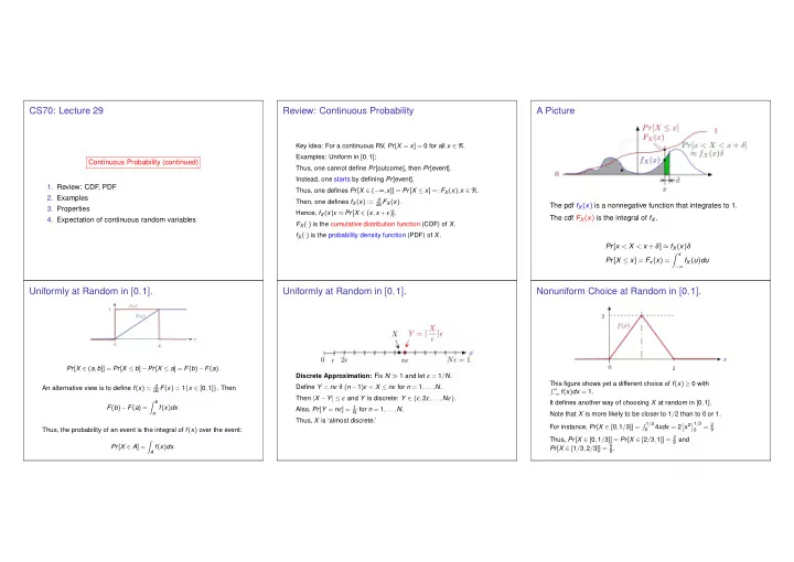
A Picture

The pdf fX(x) is a nonnegative function that integrates to 1. The cdf FX(x) is the integral of fX. Pr[x < X < x +δ] ≈ fX(x)δ Pr[X ≤ x] = Fx(x) =

x

−∞ fX(u)du

Uniformly at Random in [0,1].

Pr[X ∈ (a,b]] = Pr[X ≤ b]−Pr[X ≤ a] = F(b)−F(a). An alternative view is to define f(x) = d

dx F(x) = 1{x ∈ [0,1]}. Then

F(b)−F(a) =

b

a f(x)dx.

Thus, the probability of an event is the integral of f(x) over the event: Pr[X ∈ A] =

A f(x)dx.

Uniformly at Random in [0,1].

Discrete Approximation: Fix N ≫ 1 and let ε = 1/N. Define Y = nε if (n −1)ε < X ≤ nε for n = 1,...,N. Then |X −Y| ≤ ε and Y is discrete: Y ∈ {ε,2ε,...,Nε}. Also, Pr[Y = nε] = 1

N for n = 1,...,N.

Thus, X is ‘almost discrete.’

Nonuniform Choice at Random in [0,1].

This figure shows yet a different choice of f(x) ≥ 0 with

∞

−∞ f(x)dx = 1.

It defines another way of choosing X at random in [0,1]. Note that X is more likely to be closer to 1/2 than to 0 or 1. For instance, Pr[X ∈ [0,1/3]] =

1/3

4xdx = 2

x21/3

= 2

9. Thus, Pr[X ∈ [0,1/3]] = Pr[X ∈ [2/3,1]] = 2

9 and

Pr[X ∈ [1/3,2/3]] = 5

9.

SLIDE 2

General Random Choice in ℜ

Let F(x) be a nondecreasing function with F(−∞) = 0 and F(+∞) = 1. Define X by Pr[X ∈ (a,b]] = F(b)−F(a) for a < b. Also, for a1 < b1 < a2 < b2 < ··· < bn, Pr[X ∈ (a1,b1]∪(a2,b2]∪(an,bn]] = Pr[X ∈ (a1,b1]]+···+Pr[X ∈ (an,bn]] = F(b1)−F(a1)+···+F(bn)−F(an). Let f(x) = d

dx F(x). Then,

Pr[X ∈ (x,x +ε]] = F(x +ε)−F(x) ≈ f(x)ε. Here, F(x) is called the cumulative distribution function (cdf) of X and f(x) is the probability density function (pdf) of X. To indicate that F and f correspond to the RV X, we will write them FX(x) and fX(x).

Pr[X ∈ (x,x +ε)]

An illustration of Pr[X ∈ (x,x +ε)] ≈ fX(x)ε: Thus, the pdf is the ‘local probability by unit length.’ It is the ‘probability density.’

Discrete Approximation

Fix ε ≪ 1 and let Y = nε if X ∈ (nε,(n +1)ε]. Thus, Pr[Y = nε] = FX((n +1)ε)−FX(nε). Note that |X −Y| ≤ ε and Y is a discrete random variable. Also, if fX(x) = d

dx FX(x), then FX(x +ε)−FX(x) ≈ fX(x)ε.

Hence, Pr[Y = nε] ≈ fX(nε)ε. Thus, we can think of X of being almost discrete with Pr[X = nε] ≈ fX(nε)ε.

Example: CDF

Example: hitting random location on gas tank. Random location on circle. y 1 Random Variable: Y distance from center. Probability within y of center: Pr[Y ≤ y] = area of small circle area of dartboard = πy2 π = y2. Hence, FY(y) = Pr[Y ≤ y] =    for y < 0 y2 for 0 ≤ y ≤ 1 1 for y > 1

Calculation of event with dartboard..

Probability between .5 and .6 of center? Recall CDF . FY(y) = Pr[Y ≤ y] =    for y < 0 y2 for 0 ≤ y ≤ 1 1 for y > 1 Pr[0.5 < Y ≤ 0.6] = Pr[Y ≤ 0.6]−Pr[Y ≤ 0.5] = FY(0.6)−FY(0.5) = .36−.25 = .11

PDF.

Example: “Dart” board. Recall that FY(y) = Pr[Y ≤ y] =    for y < 0 y2 for 0 ≤ y ≤ 1 1 for y > 1 fY(y) = F ′

Y(y) =

   for y < 0 2y for 0 ≤ y ≤ 1 for y > 1 The cumulative distribution function (cdf) and probability distribution function (pdf) give full information. Use whichever is convenient.

SLIDE 3

Target U[a,b] Expo(λ)

The exponential distribution with parameter λ > 0 is defined by

fX(x) = λe−λx1{x ≥ 0} FX(x) = 0, if x < 0 1−e−λx, if x ≥ 0.

Note that Pr[X > t] = e−λt for t > 0.

Some Properties

1. Expo is memoryless. Let X = Expo(λ). Then, for s,t > 0,

Pr[X > t +s | X > s] = Pr[X > t +s] Pr[X > s] = e−λ(t+s) e−λs = e−λt = Pr[X > t]. ‘Used is a good as new.’

2. Scaling Expo. Let X = Expo(λ) and Y = aX for some a > 0. Then

Pr[Y > t] = Pr[aX > t] = Pr[X > t/a] = e−λ(t/a) = e−(λ/a)t = Pr[Z > t] for Z = Expo(λ/a). Thus, a×Expo(λ) = Expo(λ/a). Also, Expo(λ) = 1

λ Expo(1).

Expectation

Definition: The expectation of a random variable X with pdf f(x) is defined as E[X] =

∞

−∞ xfX(x)dx.

Justification: Say X = nδ w.p. fX(nδ)δ for n ∈ Z. Then, E[X] = ∑

n

(nδ)Pr[X = nδ] = ∑

n

(nδ)fX(nδ)δ =

∞

−∞ xfX(x)dx.

Indeed, for any g, one has

g(x)dx ≈ ∑n g(nδ)δ. Choose

g(x) = xfX(x).

Examples of Expectation

1. X = U[0,1]. Then, fX(x) = 1{0 ≤ x ≤ 1}. Thus,

E[X] =

∞

−∞ xfX(x)dx =

1 0 x.1dx =

x2 2 1

0 = 1

2.

2. X = distance to 0 of dart shot uniformly in unit circle. Then

fX(x) = 2x1{0 ≤ x ≤ 1}. Thus, E[X] =

∞

−∞ xfX(x)dx =

1 0 x.2xdx =

2x3 3 1

0 = 2

3.

SLIDE 4

Examples of Expectation

3. X = Expo(λ). Then, fX(x) = λe−λx1{x ≥ 0}. Thus,

E[X] =

∞

0 xλe−λxdx = −

∞

0 xde−λx.

Recall the integration by parts formula:

b

a u(x)dv(x)

=

u(x)v(x)

b

a −

b

a v(x)du(x)

= u(b)v(b)−u(a)v(a)−

b

a v(x)du(x).

Thus,

∞

0 xde−λx

= [xe−λx]∞

0 −

∞

0 e−λxdx

= 0−0+ 1 λ

∞

0 de−λx = − 1

λ . Hence, E[X] = 1

λ .

Linearity of Expectation

Theorem Expectation is linear. Proof: ‘As in the discrete case.’ Example 1: X = U[a,b]. Then (a) fX(x) =

1 b−a1{a ≤ x ≤ b}. Thus,

E[X] =

b

a x

1 b −adx = 1 b −a x2 2 b

a = a+b

2 . (b) X = a+(b −a)Y,Y = U[0,1]. Hence, E[X] = a+(b −a)E[Y] = a+ b −a 2 = a+b 2 . Example 2: X,Y are U[0,1]. Then E[3X −2Y +5] = 3E[X]−2E[Y]+5 = 31 2 −21 2 +5 = 5.5.