SLIDE 1
DNA Short Tandem Repeats
Organism
SLIDE 2
DNA Short Tandem Repeats
Organ
SLIDE 3
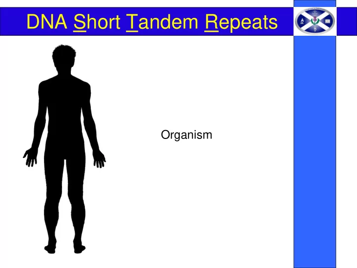
DNA Short Tandem Repeats
Cell
SLIDE 4 Weights
- 1kg – a bag of sugar
- 1g – paper clip
- 1mg (milligram) 0.001g – brain of a bee
- 1µg (microgram) 0.000001g weight of a
bacterium
- 1ng (nanogram) 0.000000001g a millionth
- f a grain of salt - recommended input to
profiling
- 1pg (picogram) 0.000000000001g 6pg of
DNA from each cell
SLIDE 5 Cells
- We lose about 30,000-40,000 skin cells an
hour
- In a year, you lose about 8lbs of cells
- “Where do they all go? The dust that collects
- n your tables, TV, windowsills and on those
picture frames that are so hard to get clean is made mostly from dead human skin cells. In
- ther words, your house is filled with former
bits of yourself.”
- About 10,000 will fit on the head of a pin
- Current DNA technology can profile one cell
SLIDE 6
DNA Short Tandem Repeats
Nucleus
SLIDE 7
DNA Short Tandem Repeats
Chromosomes
SLIDE 8
DNA Short Tandem Repeats
DNA
SLIDE 9
DNA Short Tandem Repeats
Locus
SLIDE 10
DNA Short Tandem Repeats
STR
SLIDE 11
DNA Short Tandem Repeats
SLIDE 12
DNA Short Tandem Repeats
Allele
SLIDE 13
DNA Short Tandem Repeats
Allele 5 3
SLIDE 14
DNA Short Tandem Repeats
Locus is important FGA 3 D3 3
SLIDE 15 DNA Short Tandem Repeats
A D3 vWA D16 D2 D8 D21 D18 D19 THO1
X Y 17 18 18 11 12 18 24 12 14 29 13 17 14 9 9.3
DNA profile Locus Allele Heterozygote Homozygote
SLIDE 16 The process
- Extraction
- Quantitation
- Amplification
- Separation
- Interpretation
- Evaluation
SLIDE 17
Amplification = Multiplication
SLIDE 18
Raw data
SLIDE 19
Single source profile
SLIDE 20
One DNA component from mother, another from father Area of DNA tested Names of DNA components
SLIDE 21 Why statistics?
- DNA is NOT unique
- We look at only a few areas
- Need to know what the probability
- f finding the profile by chance is
(i.e. to give an idea of how many
- ther people may have been the
source of the profile)
SLIDE 22 Statistical estimates
= 0.1
1 in a billion 1 in 10 1 in 111 1 in 20 1 in 22,200
x x
1 in 100 1 in 14 1 in 81 1 in 113,400
x x
1 in 116 1 in 17 1 in 16 1 in 31,552
x x
SLIDE 23 Probability
- Black hair
- Blue eyes
- Beard
- Gold tooth
0.6 0.25 0.01 0.001
Probability= 0.6 x 0.25 x 0.01 x 0.001
= 0.0000015 = 1 in 666,666
SLIDE 24
Random Match Probability
R B f 0.1 0.1
RB = 0.1 x 0.1 = 0.02 = 2 in 100 x 2 = 1 in 50
SLIDE 25
Mixtures
SLIDE 26
Mixtures
SLIDE 27
?
Mixtures
SLIDE 28
?
Mixtures
SLIDE 29
?
Mixtures
SLIDE 30
?
Mixtures
SLIDE 31
Mixtures
RB RY RG BY BG GY
= 6 ‘suspect’ profiles that ‘cannot be excluded’ as contributors
SLIDE 32 How many suspects?
- With 6 possibilities at each of 15 areas
- There are 6x6x6x6x6x6x6x6x6x6x6x6x6x6x6=
- More than 60 million suspect profiles
SLIDE 33 Alleles observed on ‘outside’
D8 D21 D7 CSF D3 THO1 D13 D16 D2 D19 vWA TPOX D18 D5 FGA
13 31.2 8 10 11 10 11 12 16 17 18 6 9 9.3 11 12 11 12 13 14 17 19 25 13 14 14 15 16 8 11 12 14 15 16 12 13 21 22 24 25 13 29 31.2 32.2 8 10 11 12 11 12 16 18 6 7 8 9.3 11 12 13 9 12 13 14 17 25 13 14 14 16 18 8 11 14 16 12 13 20 21 24
SLIDE 34 D8 D21 D7 CSF D3 THO1 D13 D16 D2 D19 vWA TPOX D18 D5 FGA
13 29 31.2 32.2 8 10 11 12 10 11 12 16 17 18 6 7 8 9 9.3 11 12 13 9 11 12 13 14 17 19 25 13 14 14 15 16 18 8 11
12
14 15 16 12 13 20 21 22 24
25
Alleles observed on ‘outside’
SLIDE 35
- No. of alleles at each locus
D8 D21 D7 CSF D3 THO1 D13 D16 D2 D19 vWA TPOX D18 D5 FGA
13 29 31.2 32.2 8 10 11 12 10 11 12 16 17 18 6 7 8 9 9.3 11 12 13 9 11 12 13 14 17 19 25 13 14 14 15 16 18 8 11
12
14 15 16 12 13 20 21 22 24
25
1 3 4 3 3 5 3 5 3 2 4 3 3 2 5
SLIDE 36 No of ‘suspect’ profiles
D8 D21 D7 CSF D3 THO1 D13 D16 D2 D19 vWA TPOX D18 D5 FGA
13 29 31.2 32.2 8 10 11 12 10 11 12 16 17 18 6 7 8 9 9.3 11 12 13 9 11 12 13 14 17 19 25 13 14 14 15 16 18 8 11
12
14 15 16 12 13 20 21 22 24
25
1 3 4 3 3 5 3 5 3 2 4 3 3 2 5 1 3 6 3 3 10 3 10 3 1 6 3 3 1 10
SLIDE 37 D8 D21 D7 CSF D3 THO1 D13 D16 D2 D19 vWA TPOX D18 D5 FGA
13 29 31.2 32.2 8 10 11 12 10 11 12 16 17 18 6 7 8 9 9.3 11 12 13 9 11 12 13 14 17 19 25 13 14 14 15 16 18 8 11
12
14 15 16 12 13 20 21 22 24
25
1 3 4 3 3 5 3 5 3 2 4 3 3 2 5 1 x3 x6 x3 x3 x10 x3 x10 x3 x1 x6 x3 x3 x1 x10
No of ‘suspect’ profiles
SLIDE 38 D8 D21 D7 CSF D3 THO1 D13 D16 D2 D19 vWA TPOX D18 D5 FGA
13 29 31.2 32.2 8 10 11 12 10 11 12 16 17 18 6 7 8 9 9.3 11 12 13 9 11 12 13 14 17 19 25 13 14 14 15 16 18 8 11
12
14 15 16 12 13 20 21 22 24
25
1 3 4 3 3 5 3 5 3 2 4 3 3 2 5 1 x3 x6 x3 x3 x10 x3 x10 x3 x1 x6 x3 x3 x1 x10 = 78,732,000 ‘suspect profiles
No of ‘suspect’ profiles
SLIDE 39
D8
SLIDE 40
D8
SLIDE 41
D8
SLIDE 42 Adding ‘new’ alleles at D8
D8 D21 D7 CSF D3 THO1 D13 D16 D2 D19 vWA TPOX D18 D5 FGA
9 11 13 14 29 31.2 32.2 8 10 11 12 10 11 12 16 17 18 6 7 8 9 9.3 11 12 13 9 11 12 13 14 17 19 25 13 14 14 15 16 18 8 11
12
14 15 16 12 13 20 21 22 24
25
4 3 4 3 3 5 3 5 3 2 4 3 3 2 5 6 3 6 3 3 10 3 10 3 1 6 3 3 1 10
472,392,000 (470m) ‘suspect’ profiles
SLIDE 43
D21
SLIDE 44
D21 ‘zoom’
SLIDE 45
D21
SLIDE 46 D8 D21 D7 CSF D3 THO1 D13 D16 D2 D19 vWA TPOX D18 D5 FGA
9 11 13 14 28 29 30 31.2 32.2 8 10 11 12 10 11 12 16 17 18 6 7 8 9 9.3 11 12 13 9 11 12 13 14 17 19 25 13 14 14 15 16 18 8 11
12
14 15 16 12 13 20 21 22 24
25
4 5 4 3 3 5 3 5 3 2 4 3 3 2 5
D8 D21 D7 CSF D3 THO1 D13 D16 D2 D19 vWA TPOX D18 D5 FGA
19 11 13 14 28 29 30 31.2 32.2 8 10 11 12 10 11 12 16 17 18 6 7 8 9 9.3 11 12 13 9 11 12 13 14 17 19 25 13 14 14 15 16 18 8 11
12
14 15 16 12 13 20 21 22 24
25
4 5 4 3 3 5 3 5 3 2 4 3 3 2 5 6 10 6 3 3 10 3 10 3 1 6 3 3 1 10 1,574,640,000 (1.5 billion) ‘suspect profiles
Adding ‘new’ alleles at D21
SLIDE 47 D8 D21 CSF D3 THO1 D13 D19 TPOX D18 D5
IN 13 14 31.2 10 16 6 12 13 14 11 13 20 OUT 13 29 31.2 32.2 10 11 12 16 17 18 6 7 8 9 9.3 11 12 13 13 14 8 11 12 14 15 16 20 21 22 24 25
Alleles on inside & outside
SLIDE 48 The Likelihood Ratio = LR
Probability of this evidence if the DNA came from Mr X + unknown Probability of this evidence if it came from 2 unknowns
LR = Probability of E given Hpros Probability of E given Hdef
“… times more likely”
e.g. LR = 1/10 1/100 = 0.1 0.001 = 10
SLIDE 49
LR = 1 (1/frequency)
For single source profiles
=frequency e.g. 1/(1/10) = 10
SLIDE 50
Mixtures
SLIDE 51
R B Y G f 0.25 0.25 0.25 0.25 X p(Hp) p(Hd) LR RB 0.125 0.0469 2.67 RY 0.125 0.0469 2.67 RG 0.125 0.0469 2.67 BY 0.125 0.0469 2.67 BG 0.125 0.0469 2.67 YG 0.125 0.0469 2.67 “Mr X + unknown rather than two unknowns”
SLIDE 52
R B Y G f 0.1 0.1 0.25 0.25 Mr X p(Hp) p(Hd) LR RB 0.125 0.0075 16.67 RY 0.05 0.0075 6.67 RG 0.05 0.0075 6.67 BY 0.05 0.0075 6.67 BG 0.05 0.0075 6.67 YG 0.02 0.0075 2.67 “Mr X + unknown rather than two unknowns”
SLIDE 53
R B Y G f 0.1 0.1 0.25 0.25 Mr X p(Hp) p(Hd) LR RB 0.125 0.0075 16.67 RY 0.05 0.0075 6.67 RG 0.05 0.0075 6.67 BY 0.05 0.0075 6.67 BG 0.05 0.0075 6.67 YG 0.02 0.0075 2.67 “Mr X + unknown rather than two unknowns”
SLIDE 54
RG 33.33
“Mr X + unknown rather than two unknowns”
SLIDE 55
R B Y G f 0.01 0.1 0.2 0.5 Mr X p(Hp) p(Hd) LR RB 0.2 0.0012 166.67 RY 0.1 0.0012 83.33 RG 0.04 0.0012 33.33 BY 0.01 0.0012 8.33 BG 0.004 0.0012 3.33 YG 0.002 0.0012 1.67
“Mr X + unknown rather than two unknowns”
SLIDE 56
R B Y G f 0.01 0.1 0.2 0.5 Mr X p(Hp) p(Hd) LR RB 0.2 0.0012 166.67 RY 0.1 0.0012 83.33 RG 0.04 0.0012 33.33 BY 0.01 0.0012 8.33 BG 0.004 0.0012 3.33 YG 0.002 0.0012 1.67
“Mr X + unknown rather than two unknowns”
SLIDE 57
More complicated mixture
SLIDE 58
Second area
SLIDE 59
Second area
SLIDE 60
A B A C D D B C
Second area (locus)
A B C D
SLIDE 61
AB AC AD BC BD CD
= 6 ‘suspect’ profiles that ‘cannot be excluded’ as contributors
Second area only
SLIDE 62 AB AC AD BC BD CD RB RY RG BY BG YG 444
SLIDE 63 AB AC AD BC BD CD RB RY RG BY BG YG 444 889 444
SLIDE 64 AB AC AD BC BD CD RB RY RG BY BG YG 1,778 889 1,778 444 889 444
“X + unknown rather than two unknowns”
SLIDE 65 AB AC AD BC BD CD RB RY RG BY BG 44,444 22,222 44,444 11,111 22,222 11,111 YG 1,778 889 1,778 444 889 444
“X + unknown rather than two unknowns”
SLIDE 66 AB AC AD BC BD CD RB 88,889 44,444 88,889 22,222 44,444 22,222 RY RG BY BG 44,444 22,222 44,444 11,111 22,222 11,111 YG 1,778 889 1,778 444 889 444
“X + unknown rather than two unknowns”
SLIDE 67 AB AC AD BC BD CD RB 88,889 44,444 88,889 22,222 44,444 22,222 RY 3,556 1,778 3,556 889 1,778 889 RG 8,889 4,444 8,889 2,222 4,444 2,222 BY 17,778 8,889 17,778 4,444 8,889 4,444 BG 44,444 22,222 44,444 11,111 22,222 11,111 YG 1,778 889 1,778 444 889 444
“X + unknown rather than two unknowns”
SLIDE 68 Stochastic variation
Examples so far assume allele calls are certain, but low template samples cause new problems because of stochastic variation.
- Stochastic variation is random
variation
- Failure to reproduce results
- Leads to uncertainty
SLIDE 69
SLIDE 70
SLIDE 71
SLIDE 72
SLIDE 73
SLIDE 74
The crimestain
SLIDE 75
Standard technique
Enough sample so that no dropout is expected and peak height represents amount of DNA present (i.e. not variable)
SLIDE 76
SLIDE 77
SLIDE 78
SLIDE 79
SLIDE 80
SLIDE 81
SLIDE 82
SLIDE 83 Low Template Sample
- Stochastic variation is random
variation
- Failure to reproduce results
- Leads to uncertainty
SLIDE 84
SLIDE 85
SLIDE 86
SLIDE 87
SLIDE 88
SLIDE 89
SLIDE 90
SLIDE 91
A B C D E F G H I
SLIDE 92
SLIDE 93
SLIDE 94
SLIDE 95
SLIDE 96
SLIDE 97
SLIDE 98
A B C D E F
SLIDE 99 Dropout or dropin?
D8 D21 D7 CSF D3 THO1 D13 D16 D2 D19 vWA TPOX D18 D5 FGA
13 31.2 8 10 11 10 11 12 16 17 18 6 9 9.3 11 12 11 12 13 14 17 19 25 13 14 14 15 16 8 11 12 14 15 16 12 13 21 22 24 25 13 29 31.2 32.2 8 10 11 12 11 12 16 18 6 7 8 9.3 11 12 13 9 12 13 14 17 25 13 14 14 16 18 8 11 14 16 12 13 20 21 24
SLIDE 100
Probability of dropout and dropin
p(D) Is the probability that an allele is really there but you have not detected it. p(C) Is the probability that an allele you have detected is not from the crimestain – it is contamination
SLIDE 101 FST statistic
- FST is the programme used to
calculate the LR in this case
– Probability of dropout which is
- Dependent usually on the weight of DNA
- Which is unknown for the minor
contributors
– And the validation data do not support any p(D) for any weight of DNA – The LR being correct
SLIDE 102 Low Template Sample
- Identified by variable results, NOT
the amount of DNA
– Identifying ‘true’ sample alleles – Using peak height information
- Inclusion/exclusion of people
- Number of contributors