
SLIDE 1
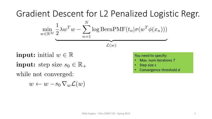
input: initial w 2 R input: initial step size s0 2 R+ while not converged: w w strwL(w) st decay(s0, t) t t + 1
1 Mike Hughes - Tufts COMP 135 - Spring 2019
You need to specify:
- Max. num iterations T
- Step size s
- Convergence threshold d
min
w∈RM
1 2λwT w −
N
X
n=1
log BernPMF(tn|σ(wT φ(xn))) | {z }
L(w)
<latexit sha1_base64="WVKZbGz9XgDFns5dP5ZCmxq463Y=">ACgHicbVFdixMxFM2MX2v9qvroy8UizIJbZ6qgCMKygvjgSpXt7kLTDplMpg2bZIYkY7fE/A7/l2/+GMF0tg+6w0h3Puzb05KRrBjU3TX1F87fqNm7d2bvfu3L13/0H/4aNjU7easgmtRa1PC2KY4IpNLeCnTaEVkIdlKcvd/oJ9+YNrxWR3bdsJkC8UrTokNVN7/gSVXuVsB5gqwJHZFO6rnx96wK0qmS40oczhKhwu824UeBGuLwms5kewAtgDbFqZO/Uu8/PQa0XgC07t+6AaTU+/OATsLmC7yGPLyRJukLcLHlynqtdCMvnrmtNiXCfLaBZ/3B+kw7QKugmwLBmgb47z/E5c1bSVTlgpizDRLGztzRFtOBfM93BrWEHpGFmwaoCKSmZnrDPTwLDAlVLUOW1no2L8rHJHGrGURMjdzmsvahvyfNm1t9WbmuGpayxS9aFS1AmwNm9+AkmtGrVgHQKjmYVagSxK8tuHPesGE7PKTr4Lj0TB7ORx9eTXYP9jasYOeoKcoQRl6jfbRzRGE0TR72gQPY/24jhO4hdxdpEaR9uax+ifiN/+AcCfwBM=</latexit>